# Welcome
Welcome to the Documentation section of HOLOPLOT Hub. You'll find comprehensive resources to help you understand, design, control, and deploy HOLOPLOT systems.
Welcome to the Documentation section of HOLOPLOT Hub. You'll find comprehensive resources to help you understand, design, control, and deploy HOLOPLOT systems.
## Discover HOLOPLOT
Introduction to HOLOPLOT
Understand the technology and key concepts behind HOLOPLOT
# HOLOPLOT unique capabilities
HOLOPLOT 3D Audio-Beamforming technology provides directivity control in both vertical and horizontal axes, allowing precise sound placement and optimal coverage of audience areas of any shape and siz
HOLOPLOT technology is science-based, software-driven, and hardware-enabled. We aim to deliver a comprehensive, end-to-end solution enclosing an interconnected hardware and software ecosystem. This enhances workflow and fosters seamless interoperability among system designers, content creators, and operational staff, by ensuring a consistent and efficient experience across all stages of sound, system design, deployment, and use.
One of the biggest limitations of conventional loudspeaker technology is the lack, or, limited control over sound propagation, leading to undirected sound waves, disturbing reflections, reverberations, and an inconsistent sound experience across the audience area.
HOLOPLOT 3D Audio-Beamforming technology allows you to steer sound and place it precisely where you want it by providing directivity control in both the vertical and horizontal axes. This allows for the creation of sound fields that optimally cover audience areas of any shape and size.
The HOLOPLOT Beam Optimization Algorithms ensure uniform coverage and consistent sound quality across the entire audience area, making every seat the best seat. With the high-resolution control of individually driven transducers per array, the sound level and frequency distribution are finely adjusted for optimal uniformity, significantly reducing the need for extensive commissioning and tuning.
### Constant SPL and STI
HOLOPLOT Matrix Arrays produce parallel wavefronts, also known as plane waves, that are flat, parallel, and travel in a single direction. In theory, the level across the direction of propagation is constant, although air absorption and other physical effects minimally affect the level over distance in practice.
In applications where speech intelligibility is the main design criterion, a system like HOLOPLOT presents several unique selling points (USPs) that, by themselves or in combination, increase the Speech Transmission Index (STI).
HOLOPLOT ensures that sound is evenly distributed across the entire audience area, avoiding hotspots and dead zones, and maintaining a consistent level and frequency response throughout. By tailoring the sound beam to the shape of the audience area, the system reduces unwanted reflections and reverberation, greatly enhancing Speech Transmission Index (STI).
### Multiple content zones from a single array
Multiple Zones
A single HOLOPLOT Matrix Array can simultaneously produce multiple sound fields (whether generated using 3D Audio-Beamforming or Wave Field Synthesis) with their own content, equalization, level, and shape.
With 3D Audio-Beamforming, we can create multiple distinct sound zones, allowing different venue areas to receive different audio content. Leveraging the advantages of HOLOPLOT's cloud-based optimization engine, each beam's coverage, level, and spectral homogeneity are optimized for every zone while minimizing sound spill between zones. This ensures precise and clear audio delivery tailored to each specific area.
This unique feature provides excellent value in functional applications and unprecedented creative potential to utilize a space for multiple different experiences.
### Focused content and targeted experiences
Virtual Sources Focused Content
HOLOPLOT's 3D Audio-Beamforming and Wave Field Synthesis technologies enable the creation of complex, immersive audio experiences. By utilizing Virtual Sources positioned in front of the array or small Coverage Beams, sound fields can be precisely targeted to specific locations within the venue, delivering tailored audio experiences to small groups or even individual audience members. The audio they hear will vary depending on their location in the venue.
This advanced capability offers a significantly broader creative sonic palette compared to traditional loudspeaker systems, allowing for the design of soundscapes that enable listeners to embark on an explorative auditory journey and feel fully immersed in the experience.
### Concealment
HOLOPLOT products blend effortlessly into their surroundings without compromising on performance. Our arrays can be fully hidden behind fabric, acoustically transparent carbon fiber panels, or LED screens.
Using 3D Audio-Beamforming to direct sound energy, the array can be flat or tilted with the screen, allowing for seamless architectural integration.
Proprietary compensation algorithms retain the characteristic clarity of sound of X1 by compensating for the angle-dependent and frequency-dependent transmission loss created by an obstructing screen. The effects can be described similarly to those of a directional-dependent, spatial EQ.
The straight shape of a Matrix Array arrangement keeps all sound sources (drivers) at a constant distance from an LED screen structure. As a result, the transmission loss in a certain direction is the same for all drivers, allowing a uniform compensation across the array.
HOLOPLOT offers the option of applying a custom 3D compensation FIR filter to each loudspeaker to enhance the performance of the arrays behind a projection panel or LED screen.
### Reflections and virtual acoustics
Virtual Sources enhance sound distribution and create immersive audio experiences. By using 3D Audio-Beamforming or focussed Virtual Sources, HOLOPLOT arrays can concentrate acoustic energy at specific reflective surfaces within a venue. This controlled redirection of sound waves enables the system to actively excite areas that otherwise pose a challenge to the system's performance.
Virtual Sources can add a layer of creativity to the system and show design. By carefully designing these reflections to arrive from different directions compared to the direct sound from the array, the illusion can be created that sound emanates from various surfaces around the venue. This technique can enhance the sense of envelopment and depth, making the sound feel more natural and immersive. For instance, Virtual Sources can contribute to the early reflections or reverberation to simulate the acoustics of a grander, more resonant space, enriching the overall experience for the audience.
### Overcoming poor room acoustics and minimizing reverb
Excessive reverberation can blur speech intelligibility and degrade audio quality in spaces with challenging acoustics. HOLOPLOT’s technology addresses this by directing sound waves to precisely where they are needed, minimizing interactions with reflective surfaces that could cause unwanted reflections and echoes. The system’s ability to create highly directional beams means that energy is focused on the audience rather than dispersing throughout the room, significantly reducing the chances of sound bouncing off walls, ceilings, and other surfaces.
This adaptability ensures that the audio remains clear and intelligible even in rooms with poor acoustics. Compared to traditional acoustic treatment, this comprehensive approach to managing room acoustics and reverb demonstrates HOLOPLOT’s capability to transform suboptimal spaces into venues with exceptional sound quality.
### Digitally programmable
HOLOPLOT's digitally programmable nature offers significant advantages in terms of flexibility and precision. The system can be configured and adjusted via software, allowing for real-time preset changes that adapt to new venue conditions or use cases without the need for physical reconfiguration of the system. This flexibility is highly beneficial for venues that host different types of events, each requiring different acoustic settings. By simply loading a different preset configuration, a concert hall can seamlessly transition from an optimal setup for a classical music performance to one suitable for a rock concert or a speech. This adaptability saves time and resources and ensures that the audio experience is always tailored to the specific requirements of each event for optimal sonic results.\
\
HOLOPLOT software updates continually enhance system performance and introduce new features. This ongoing improvement and adaptability underscore the significant advantages of a digitally programmable sound system in delivering superior and consistent audio experiences.
### Reduce noise breakouts
A HOLOPLOT system significantly reduces noise and improves noise pollution, important concerns in urban areas and multi-purpose venues. The system uses advanced 3D Audio-Beamforming technology to direct sound exactly where it's needed, minimizing the spread of sound into surrounding areas. By concentrating the acoustic energy on the audience area and avoiding unnecessary dispersion, HOLOPLOT reduces the amount of sound that escapes the intended zone, preventing noise from reaching neighboring spaces. This precise control is especially useful in places like theaters, conference centers, and mixed-use buildings, where different activities occur simultaneously and maintaining sound isolation is crucial.
Furthermore, HOLOPLOT's capability to create directed and tailored beams for specific audiences also helps in decreasing overall noise pollution. HOLOPLOT arrays benefit from the baffle effect, which effectively reduces the rear radiation of mid to low-mid frequencies. This effect is achieved by stacking Audio Modules horizontally and vertically, increasing the dimensions of the array which blocks sound that would otherwise radiate backwards. As a result, the rear sound energy is significantly reduced, preventing it from contributing to noise pollution in areas behind the speakers. This dual advantage of precise beamforming and reduced rear radiation ensures that HOLOPLOT systems deliver high-quality sound to the intended audience while minimizing the acoustic impact on the surrounding environment. This enhances overall noise management and compliance with noise control regulations.
# HOLOPLOT technology
This page explores the evolution of sound technology and highlights what sets HOLOPLOT apart.
This page offers an in-depth look at the evolution of sound technology and clearly highlights the distinctive features that set HOLOPLOT apart from other sound system solutions. You will learn about the core technological foundations underpinning our Matrix Arrays, which define and distinguish HOLOPLOT in the audio industry.
## The evolution of Sound Control
### Point sources
When a loudspeaker produces sound, its radiation pattern is determined by its shape, size, number of drivers, and properties. A point source loudspeaker produces a spherical wave that spreads equally in every direction. These wavefronts form an acoustic wave field that expands as it spreads through space and time. The energy of this wave is initially concentrated at the point source, but as it travels outward, its energy is spread over the surface of the spherical wavefronts, effectively reducing the energy as it expands. This results in a Sound Pressure Level (SPL) loss of 6dB for every doubling per distance. The rapid decline causes point sources to deliver an uneven acoustic coverage of an audience area. This is visually represented in the picture below, where the SPL level of the point source is represented as a color bar. A hot color represents a loud level, whereas a cold color represents a quiet level. Note that, although only the frontal radiation is shown in the picture below, the audio wavefronts propagate in all directions equally.
Point sources: Uncontrolled sound propagation – Single Loudspeaker with a fixed position Sound propagation direction based on mounting position & direction
By altering the shape of the sound source, the spatial and directional properties of the sound field it produces can be manipulated. One way to accomplish this is by using a loudspeaker horn, which generates a directional wave that confines the speaker's radiation range to a particular dispersion. This technique is especially effective in the high frequencies (HF) range.
### **Line arrays**
Another way of changing the radiation pattern is by combining multiple loudspeakers and relying on acoustic summation or cancellation from the individual transducers, forming a specific radiation pattern for the combination of them all. Signal processing also allows the manipulation of a sound field's spatial and directional properties. One way this is achieved is by applying appropriate processing to each driver's signal, which can alter a speaker array's radiation pattern, also called directivity. This process is known as digital beam steering.
Line arrays are speaker systems that use a vertical arrangement of transducers. These transducers have a wide horizontal and narrow vertical dispersion angle, offering dynamic control over the vertical radiation pattern, effectively controlling the level and propagation. However, they offer no control over the horizontal axis. Since the transducers are arranged vertically, beam steering is possible only on the vertical axis.
Line Array: Sound control in the vertical plane
### **HOLOPLOT Matrix Arrays**
The HOLOPLOT Matrix Array takes the concept of sound control to the next level by enabling 3D sound field manipulation. The HOLOPLOT Matrix Array comprises horizontally and vertically stacked Audio Modules, bringing full scalability to system performance and project needs. Each Audio Module contains a series of loudspeaker drivers arranged in a multi-layered two-dimensional design for the case of X1, or a single-layer two-dimensional design for X2. Each driver is processed and amplified individually, allowing for control in both the horizontal and vertical axes.
The radiation pattern of a HOLOPLOT Matrix Array can be defined and controlled very precisely in the vertical and horizontal plane. This allows for the creation of tailored sound fields with highly optimized coverage in terms of level and spectral homogeneity. This advanced and unique sound field manipulation presents considerable advantages compared to beam steering.
HOLOPLOT Matrix Arrays: Advanced Sound Control in 3D
The three-dimensional control capabilities of HOLOPLOT Matrix Arrays are powered by two different soundfield generation techniques - 3D Audio-Beamforming and Wave Field Synthesis.
HOLOPLOT's technology engine pillars
## 3D Audio-Beamforming
3D Audio-Beamforming is an advanced audio processing technique that uses an array of speakers to direct and control the propagation of sound waves in three-dimensional space. By controlling each driver's signal's relative phase and amplitude, a well-defined radiation pattern can be created by constructive interference in specific directions and destructive interference in other directions.
HOLOPLOT’s beamforming algorithms allow Matrix Arrays to be configured in two different ways.
The first one is a parametric approach where the shape of the beam is defined by a set of parameters, such as opening and steering angle. The second method uses an optimization engine to obtain an optimum coverage pattern.
### Coverage Beams
Coverage Beam
A Coverage Beam is fully tailored to the geometry of the targeted zone, providing very uniform coverage and high spectral consistency at the predefined audience area compared with traditional beamforming loudspeakers or line arrays. By utilizing digital soundfield control on both axes and directing sound where needed, reflections and spills are minimized.
Using HOLOPLOT Plan, HOLOPLOT's sound system design software, a 3D model of the space or venue, along with the array set-up positions, allows the system designer to precisely define which audience areas need to be covered by each array. Additionally, the designer can identify and define boundaries or zones that should be actively avoided by the array, such as balcony fronts or other reflective surfaces. This helps to ensure optimal sound coverage by **avoiding unwanted reflections** or interference.
For Coverage Beams, the system design follows an audience-centric approach by defining target and avoidance areas as the main design criteria. Coverage Beams are optimized to achieve the **desired** **SPL distribution** and keep a **consistent spectral homogeneity** across the predefined audience areas, ensuring everyone in the audience has the same auditory experience.
Coverage Beams are optimized in the cloud using cutting-edge algorithms that further take advantage of the 3D Audio-Beamforming capabilities of the Matrix Array. Up to five Coverage Beams can be deployed from the same Matrix Array simultaneously, irrespective of the size of the array (5 for X1, 4 for X2). The calculation of Coverage Beams relies on an internet connection.
### Parametric Beams
Parametric Beams
A Parametric Beam is a beamforming technique used to control the radiation pattern of a Matrix Array by using a set of geometric parameters. When a HOLOPLOT array emits a Parametric Beam, its direction (i.e., vertical/horizontal steering angle) and width (i.e., vertical/horizontal opening angle) are defined relative to the physical position and orientation of the array.
Parametric Beams allow for easy 3D control of the directional characteristics of an array, as compared to Coverage Beams. The design and calculation of Parametric Beams is done using HOLOPLOT Plan software locally, which is a simplified method but lacks the optimized level and spectral homogeneity benefits. However, it offers a quick and easy way to design and deploy beams within the array.
Up to 8 Parametric Beams can be deployed from the same Matrix Array simultaneously, irrespective of the size of the array. The calculation of Parametric Beams does not rely on an internet connection.
## Wave Field Synthesis
### Virtual Sources
Virtual Sources
Wave Field Synthesis (WFS) is a cutting-edge sound reproduction technology designed for spatial audio. It simulates and synthesizes virtual acoustic environments using a large number of loudspeakers arranged in a Matrix Array. The key innovation of WFS is its ability to reconstruct sound so that it appears to originate from a specific virtual starting point, known as a Virtual Source. This allows for a highly realistic and immersive audio experience, where the location of the sound source can be perceived accurately from any position within the listening area.
Unlike conventional sound reproduction techniques like stereo and surround sound, Wave Field Synthesis (WFS) does not depend on stereophonic principles, which create an acoustic illusion known as "phantom sources" in a small area (the sweet spot) at the center of the loudspeaker setup. Instead, WFS allows listeners to experience accurate localization of virtual sound sources from any position within the reproduced sound field. This means that WFS provides consistent spatial audio perception throughout the listening area. Additionally, WFS offers the highest spatial resolution among all spatial rendering techniques, delivering an unparalleled immersive audio experience.
The position of Virtual Sources in HOLOPLOT Plan can be defined using global, local, or angle coordinates, allowing them to be placed either behind or in front of the Matrix Array. Virtual Sources positioned behind the array are "visible" and correctly perceived within the audience area defined by the Field Of View (FOV). Listeners within the FOV can move freely while still accurately perceiving the location of these Virtual Sound sources. Conversely, when Virtual Sources are placed in front of the MatrixArray, the audio wavefronts from all transducers in the Matrix Array constructively add to the Virtual Source, also known as a Focus Source, resulting in a relatively high sound level compared to the rest of the listening area.
Virtual Sources are a powerful tool for creating in-field localization, targeted reflections, and special effects at specific listener positions, significantly enhancing the creative capabilities of system designers.
{% hint style="info" %}
Start working with 3D Audio Beamforming and Wave Field Synthesis in [HOLOPLOT Plan](/holoplot-plan/getting-started)
{% endhint %}
# HOLOPLOT OS
HOLOPLOT OS 2.0 is the intelligent software engine for any HOLOPLOT system. It coordinates Audio Modules to create Matrix Array systems of any size, supported by both HOLOPLOT Plan and HOLOPLOT Contro
HOLOPLOT OS is the intelligent software engine for any HOLOPLOT system. It coordinates Audio Modules to work together, creating Matrix Array systems of any size, and is enabled by both HOLOPLOT Plan and HOLOPLOT Control.\
\
This integration ensures a seamless process from planning to implementation, streamlining your tasks and enhancing overall efficiency.
## Key concepts
The following chart provides an overview of key concepts in HOLOPLOT OS. As you will see in more detail in the next section, some of these concepts are defined within HOLOPLOT Plan during the system design phase, while others are defined in HOLOPLOT Control during the operational stage.
Key Concepts of OS 2.4
## System
A system is the overall encompassing entity that holds all the information for operating a HOLOPLOT sound system. It is associated with HOLOPLOT Controller(s). HOLOPLOT Audio Modules connect via network to a single system at a time. A system has an **operational state**, **settings**, and **projects**.
### Operational state
As the name suggests, this reflects the system's current operational status, including the active project, system gain, and mute statuses.
Learn more at [Operating the system](/holoplot-control/operating-the-system)
### Settings
Those settings are shared throughout the system. For example, the chosen audio over IP standard – Dante or Ravenna, available network audio streams, and network settings.
{% hint style="info" %}
Learn more at [Configuring the system](/holoplot-control/configuring-the-system)
{% endhint %}
### Projects
Projects contain most of the information on how Audio Modules should behave. We will delve into more detail in the next section.
## Project components
The structure of a project significantly impacts both the system design and system operation stages. To illustrate this, we will examine a fictional and simplified system design of a concert venue.
A project has:
Components of a Project for a Concert Venue
### Arrays and Audio Modules
Physical representation of HOLOPLOT Audio Modules. Multiple Audio Modules are grouped into arrays.
{% hint style="info" %}
Learn more at [Arrays and modules](/holoplot-api/documentation/arrays-and-modules) and [Device health](/holoplot-api/documentation/device-health)
{% endhint %}
### Beams
{% hint style="info" %}
Learn more at [Working with beams](/holoplot-plan/working-with-beams)
{% endhint %}
At this level, the basic properties of beams, including beam type, optimization parameters, Parametric Beam parameters, and connection to Audio Modules and arrays are defined.
In the example above, we have 05 distinct beams. If we examine **left coverage**, it would be a Coverage Beam that is connected to the left array.
Left Coverage Beam
{% hint style="info" %}
Learn more at [Working with beams](/holoplot-plan/working-with-beams) and [Tuning beams in Control](/holoplot-control/operating-the-system/tuning-beams-in-control)
{% endhint %}
### Audio inputs
These are the interfaces between the Dante or Ravenna channels and streams to the beams. Each beam can have different audio input mappings based on the preset layer.
In the example above, we have 03 audio inputs that reflect how the signal will flow into the system.
### Environmental conditions
Those are defined and used for the optimization of beams. This is combined at the preset layer level.
### Preset layers
Preset layers serve as the foundational elements of a preset, grouping together beams that function in unison. This layer also handles the mapping of beams to audio inputs, as well as EQ, gain, and delay alignments and is associated with environmental conditions.
{% hint style="success" %}
A Beam's tuning is linked to the Preset Layer and environmental conditions. This means each Beam will have different Gain, Delay, and EQ values for each associated Preset Layer and Environmental Condition.
{% endhint %}
#### Main system
The **main system** preset layer in the above project consists of 03 beams connected to two audio inputs and two environmental conditions. The front fill beam receives its audio signal from both the left (01) and right (02) inputs.
Preset Layer Main System
#### Bar downmix
With this preset layer, we can independently activate a different set of beams to receive a downmix from the left (01) and right (02) inputs.
Preset Layer Bar Downmix
#### Bar independent
This preset layer takes the same beam as the previous one but assigns it to a different audio input. It can be used to send independent audio.
Preset Layer Bar Independent
#### Balcony downmix
This preset layer exemplifies an optional venue occupancy. Perhaps the under-balconies are not used in some concerts.
Preset Layer Under Balcony Downmix
{% hint style="info" %}
Learn more at [Routing streams](/holoplot-control/operating-the-system/routing-streams)
{% endhint %}
### Presets
Presets are groups of preset layers that form a functional system state that users can switch during operation. Let's look at some of the examples. We have four presets on the project:
* **Full system**: All beams are engaged
* **Main system w/o under balcony:** All beams without the under balcony
* **Main system & independent bar**: The main system operates independently from the bar
* **Main system w/o under balcony & independent bar**: Main system without under balcony, and bar operating independently
From an overview, they are presented like this:
Preset Full System
When active in the system, this is a more accurate representation of what they are doing:
Preset Full System
This approach simplifies operations for a front-of-house or system technician. Only two iudio Inputs (left and right) are needed to drive the entire system. A HOLOPLOT system handles EQ, gain, and delay settings.
Another example with the **main system & independent bar** preset:
Preset Main System & Independent Bar
The preset consists of 03 preset layers, with one key difference from the previous example: the "bar downmix" and "bar" in this one. The main distinction between the two presets is that the "bar coverage" beam now has an independent audio input (bar).
Presets Main System and Independent Bar
{% hint style="success" %}
HOLOPLOT Plan checks the total number of available and used beam slots per Audio Module at two stages: first on the preset layer and then at the preset level.
Preset layers and presets are considered valid only if the count of beams per array does not exceed the specified limits. In the case of a preset, all beams in the assigned preset layers are considered.
{% endhint %}
{% hint style="info" %}
Learn more at [Working with presets](/holoplot-plan/working-with-presets) and [Changing a preset](/holoplot-api/examples/changing-a-preset)
{% endhint %}
# Audio signal flow
This page explains how audio signal flows from the AoIP standards to HOLOPLOT's Audio Modules in OS 2.0.
This page explains how audio signal flows from the AoIP standards to HOLOPLOT's Audio Modules. We will continue using the same project example from the previous page, and will examine one preset in particular.
## Main components
The chart below explains the main components and their relationships: Audio inputs, beams, modules/arrays, and AoIP channels and streams. Here is a quick recap:
Signal Flow
**Beams, arrays, and modules**
A group of modules forms an array. Beams are connected to Audio Module(s). Audio Modules can have multiple beams, as exemplified by the Audio Modules in the front fill array. Each beam has its own individual DSP, including user-adjustable gain, delay, and EQ.
**Audio inputs, beams, and presets**
Beams are connected to audio inputs on preset layers/presets. Meaning, that their assignment can vary depending on the needs.
You can connect multiple beams to the same audio input and multiple audio inputs to the same beam. The connection between audio inputs and beams can have an optional gain value, which is set by default to 0 dBFS.
**AoIP channels and streams and audio inputs**
The previous two topics are defined inside HOLOPLOT Plan. The actual connection between your Dante or Ravenna audio channels and audio inputs happens inside HOLOPLOT Control. As the example above shows, an audio input can be fed from multiple sources.
## Audio controls and metering
Different places in the audio flow can be monitored and controlled in HOLOPLOT OS with HOLOPLOT Control.
### Audio controls
You can mute/unmute, solo/unsolo, adjust gain and delay, and apply EQs on the beam level.
On the system level, you can mute/unmute, adjust the gain, and apply EQs.
### Metering
There are meters for outputs and inputs. Outputs are modules, arrays, and system. Inputs are beams.
{% hint style="info" %}
Learn more about at [#metering](#metering "mention")
{% endhint %}
## Putting it all together
Now that the audio flow concepts are laid out let's examine some examples.
The chart above shows what audio inputs, beams, and modules will receive audio from the AoIP channel DANTE 01. Remember that each beam has individual DSPs and will process that signal accordingly.
We can take it one step further, and solo one of the beams. This is especially useful for tuning and debugging.
# Product family
### The X1 series
The ultimate sound system for large-scale live entertainment applications
X1 Matrix Array Audio in new dimensions
The range comprises two variants of the X1 Matrix Array, the Modul 96 (MD96) full range and the Modul 80-S (MD80-S), which is a full range loudspeaker with integrated subwoofer. Let’s have a look at their components and design.
#### MD96
* **64x** 1.3-inch high-frequency soft-dome drivers coupled with individual waveguides
* **16x** 5-inch low-frequency cone driver in individual dual-ported chambers
* **1x** 18-inch sensor-controlled subwoofer with two high energy, high-density neodymium-iron-boron magnets in a bandpass enclosure with air-flow optimized ports.
#### S21
* A 21-inch sensor-controlled high-performance subwoofer in a bass-reflex enclosure with four ports
* Single-channel digital subwoofer amplifier module with differential pressure sensor and onboard zero-latency-DSP
### The X2 series
Same control, new dimensions: Optimized for speech applications and integration in challenging acoustic environments.
MD30
* Best-in-class intelligibility for speech applications - the logical subsequent development in HOLOPLOT's ongoing commitment to delivering unrivaled sound control.
* From auditoria and conference events to worship spaces and public transportation hubs, X2's compact form factor makes HOLOPLOT technology accessible for more applications than ever.
***
### Datasheets and User Manuals
Find more detailed information for all products in [downloads](broken://spaces/z66RY3xb2z8uBaNIH6K1).
# HOLOPLOT system design
Learn the specifics of designing with HOLOPLOT systems and beams, including how to control and shape sound patterns for optimal effects
In this guide, you will learn the specifics of designing with HOLOPLOT systems and beams, including how to control and shape sound patterns for optimal effects. You will discover the different types of beams available and learn how to use them to achieve the best results in your projects.
Jump to any of the steps or click on the next section at the bottom of this page.
System design best practices
This resource provides the essential principles and key considerations for effectively integrating HOLOPLOT systems into your projects.
# System design best practices
This resource provides you with essential principles, best practices, and key considerations for effectively integrating HOLOPLOT systems into your projects.
Jump to any of the steps or click on the next section at the bottom of this page.
{% content-ref url="/pages/h1WGj86bFxIH9qjWJP6N" %}
[Introduction to sound system design](/user-guides/holoplot-system-design/system-design-best-practices/introduction-to-sound-system-design)
{% endcontent-ref %}
{% content-ref url="/pages/QTHec46EdmEmIybWIvy2" %}
[Which HOLOPLOT product is best suited to the application?](/user-guides/holoplot-system-design/system-design-best-practices/which-holoplot-product-is-best-suited-to-the-application)
{% endcontent-ref %}
{% content-ref url="/pages/tg6fU08QmqTF9p2AI67X" %}
[How do I decide on the position of my arrays?](/user-guides/holoplot-system-design/system-design-best-practices/how-do-i-decide-on-the-position-of-my-arrays)
{% endcontent-ref %}
{% content-ref url="/pages/X5iWdzk8vZo5f4G6VBGl" %}
[What should be the size and aspect ratio of my arrays?](/user-guides/holoplot-system-design/system-design-best-practices/what-should-be-the-size-and-aspect-ratio-of-my-arrays)
{% endcontent-ref %}
# Introduction to sound system design
In this section, you will explore the key considerations for designing with a HOLOPLOT system and delve into the main performance indicators of a well-designed system.
The design process starts with a consultation with the client, allowing the designer to gain a thorough understanding of the project's requirements and intended applications. From this initial discussion, a list of design assumptions, performance targets, and engineering constraints can be compiled.
Following this, a detailed assessment should be conducted, focusing on key acoustic performance targets such as:
* Loudness
* Fidelity
* Uniformity
* Intelligibility
* Localization
### Loudness
{% hint style="success" %}
* Signal-to-noise ratio
* Artistic requirements
* Adequate levels even at the last seat
* Loudness homogeneity across all audience areas
* Overall values highly dependent on application
{% endhint %}
Many might assume that the louder a sound system, particularly in live entertainment, the better it performs. However, system designers must consider several other crucial factors.
* Uniformity of sound level is often a priority for clients wanting to ensure consistent coverage and quality across all seating areas within a venue.
* It's also vital to have a distortion-free signal reproduction. To achieve this, it's necessary to specify a system that provides ample headroom to handle all anticipated uses.
* Moreover, even a system with adequate headroom must achieve the necessary gain before feedback onstage to be fully effective. During the design phase, it is essential to evaluate onstage sound levels to ensure they meet this criterion.
The specific level requirements vary based on the application and can be influenced by factors such as:
* High ambient noise levels as a result of crowd noise or environmental noise at locations like transport hubs.
* Preferences of the artists and engineers.
* Regulations set by local authorities concerning health and safety or noise limitations at the venue's perimeter.
### Fidelity
{% hint style="success" %}
* No coloration
* No distortion
* Faithful copy of the original signal delivered to all seats
{% endhint %}
Achieving sound reproduction that remains true to the original signal is the primary objective for system engineers. This fidelity allows front-of-house (FoH) engineers to create a mix that closely resembles the studio recording. When a system introduces significant coloration, extensive post-processing becomes necessary to attain the desired sound. This aspect is particularly crucial for touring shows that aim for a consistent sound quality at every performance, irrespective of the venue's acoustical influence. The less a system is affected by room acoustics, the less need for equalization and dynamic processing.
### Uniformity
{% hint style="success" %}
* Spectral homogeneity across all receivers
* Small standard deviation
* Typically +/- 3dB
{% endhint %}
Uniformity in sound systems isn't just about consistent levels or even distribution across different areas; it also involves ensuring spectral uniformity so that all audience members have a similar auditory experience. Evaluating both uniformity and the sound level per octave band is crucial, intending to minimize the standard deviation among all listeners to within a specified tolerance, commonly ±3 dB. However, this tolerance might be broader for higher frequencies, particularly when speaker arrays must cover long distances or when environmental conditions, such as temperature and humidity, come into play.
### Intelligibility
{% hint style="success" %}
* Intelligible speech across all listeners
* Speech Transmission Index (STI)
* ISO 60268-16
{% endhint %}
Intelligibility hinges on three critical factors:
1. Signal to noise ratio (SNR): This measures the signal level against the background noise.
2. Direct to reverberant ratio: This assesses the clarity of direct sounds compared to reflected sounds.
3. Signal masking: The upward spread of masking is an acoustic phenomenon where lower-frequency sounds (maskers) make it harder to hear higher-frequency sounds (signals). This effect is more pronounced when the lower-frequency sounds increase in volume or intensity.
For optimal intelligibility, the system should be designed to maintain the sound level at each octave band significantly above the background noise—typically 10-15 dB higher. However, achieving this can be challenging in environments with inherently high background noise, such as transport hubs, stadiums, or road tunnels. In these cases, the cost and size of the system must be balanced against the potential improvement of intelligibility, keeping in mind the diminishing returns as the ear's self-protection mechanism can reduce signal intelligibility at very high volumes.
A direct sound pressure level (SPL) of 70-80 dB is generally considered ideal in quieter settings.
# Which HOLOPLOT product is best suited to the application?
This section offers insight into selecting the ideal HOLOPLOT product for your project, helping you make informed decisions.
### How are the products used in design?
{% hint style="info" %}
Find each product's datasheet and manual in the [Product Family](/introduction-to-holoplot/product-family) section
{% endhint %}
HOLOPLOT products have been designed to apply a standard modeling and simulation workflow across the product range. All commercially available products are included in [HOLOPLOT Plan](/holoplot-plan/getting-started).
### How do you decide which product to use?
Choosing the right product for your design is based on the individual use case. However, there are particular segments that each product was designed to support.
{% tabs %}
{% tab title="X1" %}
{% endtab %}
{% tab title="X2" %}
{% endtab %}
{% endtabs %}
In addition to these segments and the aforementioned acoustic parameters (see [Introduction to Sound System Design](/user-guides/holoplot-system-design/system-design-best-practices/introduction-to-sound-system-design)), the following parameters need to be considered:
#### Weight loading
When specifying a HOLOPLOT array, it's crucial to consider the weight-loading capacity of the building, structure, and rigging apparatus. For example, the X1 and X2 series Audio Modules are active, with all amplification and processing onboard, significantly increasing their overall weight. This often necessitates specialist rigging or installation advice to ensure safe deployment. Designers should be aware of the system's weight and able to offer high-level advice on feasible rigging solutions. The integration partner should provide detailed rigging plans based on the specifications from HOLOPLOT.
#### Integration/ space allocation
Whether working at the earliest stage of a construction timeline or specifying a system for a retrofit, it is imperative to ensure that you have sufficient space in a given location to deploy arrays safely and efficiently. This is particularly important when flush mounting an array into a facade; this requires sufficient depth in the wall build-up and additional space for ventilation. Access for maintenance and servicing of the module should also be taken in to consideration (see manual for instructions on access requirements).
#### Power
Power specifications must be provided to the integration partner to calculate the necessary loads. Typically, as a manufacturer, we are not responsible for providing system power calculations. However, when no integration partner is involved in the project, power calculations should be approved by a qualified engineer on the team responsible for installation and commissioning.
#### Weatherization (IP rating)
The X1 system is not IP-rated. Thus, it requires external weatherproofing for deployment in environments that expose it to conditions outside its normal operating parameters. Such environments include outdoor areas or indoor spaces with high humidity or water exposure. In contrast, the X2 system is IP55 rated, making it suitable for outdoor operations. However, if extreme weather conditions are anticipated, it is advisable to consult the manual to understand the specific exposure parameters.\
\
For the exact specifications on the above parameters, please refer to the HOLOPLOT X1 manuals found in the section: [Product Family](/introduction-to-holoplot/product-family)
# How do I decide on the position of my arrays?
Find essential insights into positioning arrays effectively and explore the unique aspects of positioning HOLOPLOT arrays compared to conventional systems.
Placeholder
Correct positioning of arrays is crucial for optimal acoustic performance, impacting sound levels, the direct-to-reverberant ratio, coverage, and sound localization. While HOLOPLOT systems can adjust for less-than-ideal speaker placements, designers should aim for the best possible locations to reduce the need for extensive processing to achieve desired performance levels.
Often, the geometry or architectural characteristics of a space dictate speaker placement. This could be influenced by an architect's initial design, space limitations, or the load-bearing capacity of existing structures, which might result in compromises.
When compromises are necessary, it’s important to evaluate the following parameters carefully:
**Is there sufficient weight-loading and space allocation for the specified arrays?**
* See the product manuals in [Product Family](/introduction-to-holoplot/product-family) for specific weight loading specifications. Make an assessment of space allocation based on the architectural model and consider visiting the site where applicable.
**What are the required beam opening angles, and can the specified array sizes achieve this across a suitable bandwidth?**
* See the chart in [Array Right Sizing](/user-guides/holoplot-system-design/system-design-best-practices/what-should-be-the-size-and-aspect-ratio-of-my-arrays#array-right-sizing) to make an assessment of the arrays steering capabilities
**What are the beam steering angles, and can these be achieved across a suitable bandwidth?**
* See the chart in [Array Right Sizing](/user-guides/holoplot-system-design/system-design-best-practices/what-should-be-the-size-and-aspect-ratio-of-my-arrays#array-right-sizing) to make an assessment of the arrays steering capabilities
**Are the steering angles likely to create problematic side lobes, potentially causing audible echoes or reflections off hard surfaces?**
* Making an assessment of the potential lobing that is inherently caused when electronically steering a beam can be assessed by calculating the the expected spatial aliasing frequency and simulating the performance to asses the impact. It's important to understand this as a designer to ensure any unwanted reflections or artefacts won't be present in the final system deployment.\
This will also provide the designer with an understanding of the expected amount of edge defraction causing smaller side lobes outside off axis of the main lobe. When taking this into consideration the following rules apply.
* At high frequencies, the directivity control is defined by the spacing between the loudspeaker drivers. In particular, reducing the spacing between drivers will improve (increase) the maximum frequency that can be controlled for beam steering or beam shaping.
* Above a certain frequency, *grating lobes* (i.e., replicas of the main lobe that radiate in a different direction) will occur due to spatial undersampling of the array (too few samples or low loudspeaker driver density) during acquisition. This frequency is known as aliasing frequency.
* A typical directivity pattern of an array is illustrated in the polar diagram below. Apart from the main lobe, also smaller *side lobes* are shown. These side lobes occur due to array diffraction. Tapering (gradually reducing) of the amplitude of the loudspeaker drivers near the edges of the array, decreases the level of these side lobes, compromising on the beam width (effectively using a narrower array) This is implemented into the HOLOPLOT optimization algorithm to reduce the level of side lobes.
Polar diagram illustrating a possible directivity pattern of an array using beam forming
{% hint style="info" %}
To avoid spatial aliasing the spacing *d* should be smaller than half the wavelength λ (Nyquist criterion) of the maximum frequency to be controlled.
{% endhint %}
**If arrays are flush mounted into walls, is there sufficient ventilation to maintain a healthy operating temperature?**
* See the product manuals in [Product Family](/introduction-to-holoplot/product-family) for specific weight-loading specifications.
**How do I ensure the correct localization of the acoustic source or visual content for the majority of the audience members?**
* To make an assessment of correct localization, we have to consider 3 main criteria: angle, level, and arrival time of the first wavefront. The aim of the designer is to achieve a plausible localization of the acoustic source. In a simple frontal mono system (single source), this is a simple concept where the position of the array should be within approximately 30 degrees of separation from the acoustic source to ensure the psychoacoustic phenomena where the listener makes up the difference between the source position and the first wavefront produced by the loudspeaker take effect. This often becomes problematic to achieve when an array needs to be located in a high position above a stage opening, causing the localization to break down for the front rows of the audience. This will often require front fills (multiple sources) to correct the localization.
### Auditory events with multiple sources
Now consider two sound sources emitting the same signal. Several auditory events can occur depending on the location and delay between the two sources:
* **Summing localization (phantom source)**\
For very short time differences (≤1 ms), summing localization occurs, where the location of the perceived sound depends on the level and time difference of the two sources at the listener position.
* **Precedence effect or 'law of the first wave front'**\
Increasing the time delay between the two sources to more than 1 ms, the perceived direction no longer changes. It sticks closely to the direction of the leading source.
* **Echoes**\
Further increasing the time delay to more than 50-80ms, the sound perception transits from one (wide) source to two sources separated in time and location as a primary auditory event and its echo.
Visualization of the three stages of auditory events with multiple sources (Kohlrausch et al., 2013).
### Echoes
The echo threshold is defined as the delay at which the secondary source is barely perceptible. The echo threshold is not a single value, but also depends on the level difference between the two arriving signals as well as their temporal and spectral structure. It varies roughly from 1 ms for short impulses to around 80 ms for more continuous sounds. The probability of hearing an echo with a speech signal is around 50 ms when the level of the lagging signal is 10 dB lower than the leading (Blauert, 1974).\
\
The figure below shows the different thresholds as measured using the standard stereophonic loudspeaker arrangement, speech presented at a rate of approximately 5 syllables per second, and the level of the primary sound approximately 50 dB at the position of the subject.
* The lowest threshold curve represents the the masked threshold.
* The next curve upwards is the echo threshold. If the delay time is less than approximately 32 ms, the level of the lagging sound can even be as much as 5 dB higher than that of the primary sound without the echo becoming audible.
* The next curve is the equal loudness curve for the primary auditory event and the echo. At a delay time of 15 ms, the reflection must be more than 10 dB stronger than the primary sound to lead to an equally loud auditory event.
* At delay times less than 50 ms, echoes are no longer perceived as annoying even if the reflection is\
considerably stronger than the primary sound. This is known as the "Haas effect," due to its description by Haas (1951).
* The level above which the primary auditory event disappears is shown in the uppermost\
curve.
A comparison of various thresholds for reflections; standard stereophonic loudspeaker arrangement (data of Haas 1951, Meyer and Schodder 1952, Burgtorf 1961, Seraphim 1961).
These fundamental principles need to be taken into consideration when designing with a HOLOPLOT system. The initial positioning of arrays can ensure that both correct time and level alignment are achievable for as large a proportion of the audience as possible.
### What is different about how you position HOLOPLOT arrays compared to conventional systems?
HOLOPLOT arrays differ from conventional speaker technology because they can be electronically steered and optimized. While it remains crucial to mount them as close to optimal positions as possible, designers enjoy greater flexibility with HOLOPLOT arrays. In contrast, conventional speaker technology is often limited by fixed dispersion patterns, where the radiation pattern is dictated by mechanical components such as horns, baffles, or waveguides that physically direct sound dispersion.
Line array technology has addressed these limitations by enabling designers to control sound in the vertical axis, creating a cylindrical wavefront. This advancement reduces energy loss over distance from the typical 6dB per doubling of distance of a point source to just 3dB per doubling of distance. This technology allows for sound to be projected over greater distances, reducing the need for multiple mounting positions and enabling larger and more varied venue shapes to be efficiently covered with sound.
The major drawback to this technology, however, is the lack of control over the horizontal axis, which results in unwanted reflections off side walls and a loss of energy over distance.
HOLOPLOT Matrix Array technology has overcome this, enabling control in both the horizontal and vertical axis. This, coupled with HOLOPLOT's proprietary optimization algorithms, has granted the ability to control the loss of energy over distance; energy loss is now primarily down to air absorption impacting the high frequencies
{% hint style="info" %}
See [Beam design best practices](/user-guides/holoplot-system-design/beam-design-best-practices) for more information on how and when to compensate for these losses and reducing reflections which drives up the direct to reflected ratio improving overall intelligibility.
{% endhint %}
### Example layouts for multi-array designs
Although a single HOLOPLOT array can cover a large area, a complete sound system often requires multiple arrays because of the size and shape of the audience areas or the presence of architectural elements blocking the sound, such as pillars, kiosks on train platforms, etc.
Using multiple, distributed sound sources in a space emitting the same signal increases the risk of echoes due to the time differences in the arrival of the direct sound. Hard reflective surfaces might also add echoes, which are ignored for now.
### Elementary design concepts
In large spaces often, multiple arrays are needed. To speed up the design process, different elementary design concepts and beam options are available:
| Design concepts and beam options | Criteria |
| -------------------------------------------------------------------------------------------------------------------------------------------------------------------------------- | ------------------------------------------------------------------------------------------------------------------------------------------------------------------------------------------------------------------------------------ |
|
Central
Face-to-Face
Transversal
Longitudinal (time-aligned)
Some combinations of the above
Long or short throw beams?
|
Geometry and size of space or venue
Sound localization
Interaction with other coverage areas
Available (ceiling) height
Shadowing by sound-blocking objects (i.e., lines of sight)
|
#### Central: Two arrays back-to-back, shooting in opposite directions.
Note that the arrival time delay increases from the center of the setup to either end. This is important if this setup is acoustically coupled to another area. Late echoes might be audible in the transition zone between the two areas.
#### Transversal: Multiple arrays in a row along a wall, shooting across the space
The spacing between the arrays depends on the horizontal opening angle. For column loudspeakers having a triangular coverage pattern the spacing shouldn’t be much larger than 10 m. For Matrix Arrays, the spacing can be increased by creating ‘virtual sound corridors’, minimizing the overlap between the adjacent sections.
An economical solution can be obtained by alternating larger and smaller arrays, having a longer and shorter throw, respectively.
#### Face-to-face: Two arrays shooting towards each other
To avoid echoes the distance between the arrays should be smaller than \~20m. Even if each beam covers only half the area, the floor reflection indirectly causes overlap and potentially delay issues.
#### Longitudinal (time-aligned): Multiple arrays along a line, shooting in the same direction.
The arrays must be time-aligned to create a coherent wavefront along the longitudinal direction. Due to the backward radiated energy (stronger for LF), a weak echo might be audible a couple of meters behind each delayed array. To minimize this effect, the delay could be set 5-10 ms shorter than what’s calculated based on the distance. The auto-delay tool in (the soon-to-be-released) HOLOPLOT Plan 2.01 will automatically take the effect of backward radiated energy into account.
To further improve the performance, high-passing or low shelving the delayed arrays can be considered. This will reduce the LF level behind the delayed arrays.
{% hint style="info" %}
Note that the arrival time delay increases from one end of the setup to the other. This is important if this setup is acoustically coupled to another area. In the transition zone between the two areas late echoes might be audible.
{% endhint %}
### **Combinations of elementary design blocks**
#### Central & longitudinal setup
This setup is particularly useful on train station platforms. The position of the two back-to-back arrays defines the ‘zero-time’ point of the setup. In case of a cross connecting tunnel or bridge between the platforms, covered by zero-delay loudspeakers, the zero-time on the platforms should be placed near the cross passage. This minimizes the risk of late echoes in the transition area between the two (weakly) acoustically coupled areas.
#### Multiple transversal
This setup is useful for covering a large area such as a mosque or baggage claim area at an airport. The size of the arrays mainly depends on the available ceiling height. The spacing depends on the type of array (see transversal setup).
#### Multiple face-to-face
In general, this setup is less favorable than the time-aligned longitudinal setup. However, it still has a use case for example if no delays can be applied due to a acoustically coupled neighboring area covered by zero-delay loudspeakers.
# What should be the size and aspect ratio of my arrays?
Determining the size of your arrays requires careful consideration. This article explores guidelines for effectively sizing arrays to attain the desired level of control.
### Right sizing of an array
When sizing an array there are some general rules you should consider; the size of the array, whether it is 1D (line) or 2D (planar), will influence the directivity capabilities of a sound source, in our case the array:
* Bigger arrays can create narrower beams compared to smaller arrays.
* At a given frequency, if the array size increases, the narrowest obtainable beam gets narrower.
* If the array size increases, the frequency at which the narrowest possible beam is obtained decreases.
It's a well-known principle that enlarging an array can boost the sound pressure level for a designated area. Specifically, doubling the size of the array typically results in a 3dB increase in sound level, although this can vary depending on the opening angles and types of beams used. We will explore this concept further through several practical examples.
In setting up an array, the aspect ratio of the target area should guide its configuration. For long and narrow spaces, the array should be dimensioned vertically longer than horizontally to best cover the area. However, if minimizing sound spill to side walls and focusing sound tightly within the area is crucial, then increasing the width of the array may be advisable to achieve a higher precision in sound distribution.
The chart below shows the relationship between array size, both horizontally and vertically, and the achievable beam opening angle, which could also be described as the minimum obtainable beam width as a function of frequency for different array lengths.
With the added variable of sound control in both the horizontal and vertical axes, it is useful to establish a set of controls to provide clear right-sizing guidance. The following case study aims to validate two rough guidelines for determining the appropriate sizing for a given coverage area. The rules are as follows:
{% hint style="info" %}
* **Doubling the size of the array gives you 3dB increase in broadband SPL**
* **To ensure consistent coverage the array needs to increase by 1 row/10m of distance throw**
{% endhint %}
As stated, these assumptions are guidelines based purely on coverage and a standard shoebox geometry where the array is throwing the length of the space. This does not take into consideration any additional control requirements that may be needed to achieve the desired intelligibility or reduce sound spill to adjacent spaces.
The below array sizing tool (see link below ) can be used to predict the minimum obtainable beam width in degrees
{% embed url="" fullWidth="true" %}
HOLOPLOT X1 Array Sizing tool
{% endembed %}
### Array sizing – Worked examples
Four common use cases will be considered to provide a more practical basis for sizing a HOLOPLOT array. In the example, a simple shoebox auditorium will be used. Here, a central array will be considered to show how SPL (dBA) changes both in level and coverage homogeneity as a result of increasing the size of the array. In these examples, a single coverage beam is used, utilizing HOLOPLOT's optimization algorithms to ensure the most desirable performance.\
\
Design criteria was as follows:\
Each array must cover the intended zone with the following homogeneity:
> * 90% coverage ±3 Broadband dBA
> * 85% coverage ±3 Octave bands (250-10,000Hz)
#### Example 1 – 1x2 centrally mounted MD96 array
> * SPL Drop: 0
> * Air absorption compensation: 0
> * Target curve: Flat
> * Phase response: Linear
> * Input Signal: AES2 (pink noise)
### Comparison across different array configurations
The data from the chart below presents the sound pressure level (SPL), homogeneity, and sound range across different array configurations of the HOLOPLOT system in a small theatre setup, broken down into three zones and a combined overview.
Here are the observed patterns and trends:
**Sound pressure level (SPL) Trend:**
Increasing SPL with larger arrays: SPL consistently increases (on average, 3dB per doubling of array size) as the array configuration increases from 1x2 to 4x2 in all zones. This indicates that more speakers in the array contribute to higher loudness levels, which can cover larger areas more effectively.
**Homogeneity (%):**
Improved homogeneity with larger arrays: Homogeneity, or the uniformity of sound distribution, improves with the size of the array in each zone. Higher homogeneity indicates a more evenly distributed sound that avoids dead spots and overly loud areas.
**Range (dBA SPL):**
Narrower range with larger arrays: The range of SPL, which indicates the variability of loudness across the zone, tends to become narrower (i.e., more consistent) with larger array configurations. This is beneficial for ensuring that all audience members experience similar sound levels.
**Summary of trends:**
1. **Loudness and coverage**: As array sizes increase, SPL and coverage (homogeneity) improve, making larger configurations preferable for larger or acoustically challenging environments.
2. **Sound consistency**: Larger arrays improve loudness and enhance the consistency of sound across different theatre zones, reducing the variability in the audience experience.
3. **Optimal configuration**: Based on the trend, the 4x2 MD96 configuration appears to be the most effective in providing high and consistent SPL, along with excellent homogeneity and a narrow SPL range, making it suitable for theaters seeking robust and uniform sound distribution.
Examining the performance of each array when optimized for a specific zone or zones, it's evident from the chart above that a 1x2 array is sufficient to cover the first 10 meters of the auditorium. It provides both sufficient SPL (95dBA broadband and 85dB at all octave bands from 250 to 10,000Hz) for most live performance use cases, with the exception of high SPL music shows. Additionally, it ensures adequate coverage for almost the entire audience, offering a consistent audio experience. A 90% broadband coverage is deemed adequate for this venue, with 85% coverage at all octave bands from 250 to 10,000Hz.
When trying to cover both zones, the 1x2 array achieves the 90% coverage threshold for the broadband dBA results but fails to meet the 85% threshold for octave bands from 4kHz and above (see chart below). All other arrays achieved this. Similarly, when assessing coverage for all three zones, the 2x2 array met the broadband coverage requirement but did not achieve the 85% ±3dB coverage at all octave bands (250-10,000Hz).
{% hint style="info" %}
The above simulations provide the basis for an initial assessment of array sizing. Use the rule of 10 meters per row for height whilst considering the SPL requirement, noting that a 3dB increase occurs when the array size is doubled. Additionally, use the HOLOPLOT array calculator to evaluate beam control. This approach allows the designer to approximate the optimal system size before running a detailed simulation.
{% endhint %}
# Beam design best practices
Learn about the different types of beams available, their applications, and the detailed design process. Designing with beams, a concept often associated with lighting involves controlling and shaping patterns for optimal effects. This principle is fundamental to the HOLOPLOT design approach. We will cover the types of beams available, where and how to use them, and the detailed process of designing sound systems with HOLOPLOT technology.
Jump to any of the steps or click on the next section at the bottom of this page.
{% content-ref url="/pages/3VNRDvaMtbK7gHVLKeKx" %}
[What are the fundamental principles of designing with beams?](/user-guides/holoplot-system-design/beam-design-best-practices/what-are-the-fundamental-principles-of-designing-with-beams)
{% endcontent-ref %}
{% content-ref url="/pages/I2g9u3LimB3D0XF4df3H" %}
[How do I set up my coverage zones and what impact does that have on my design?](/user-guides/holoplot-system-design/beam-design-best-practices/how-do-i-set-up-my-coverage-zones-and-what-impact-does-that-have-on-my-design)
{% endcontent-ref %}
{% content-ref url="/pages/mesHy7RmNfbrQsG5XNNZ" %}
[What are the different beam parameters and how do I apply them in my design?](/user-guides/holoplot-system-design/beam-design-best-practices/what-are-the-different-beam-parameters-and-how-do-i-apply-them-in-my-design)
{% endcontent-ref %}
{% content-ref url="/pages/NE23eCtivfWBSpfI1QUF" %}
[How do I apply those beams in real world applications?](/user-guides/holoplot-system-design/beam-design-best-practices/how-do-i-apply-those-beams-in-real-world-applications)
{% endcontent-ref %}
# What are the fundamental principles of designing with beams?
**What are the fundamental principles of designing with beams?**
The concept of designing with beams is more commonly associated with lighting, where mechanical shutters control the light pattern to either highlight a performer or wash the entire stage with light from the same fixture. This principle of controlling and shaping beams is fundamental to the design approach of HOLOPLOT system. This section will outline the design process using these principles, outlining the types of beams available and where and how to use them for the optimal effect.
There are two primary beam types:
**Parametric Beams**
A Parametric Beam is defined by a set of parameters allowing the adjustment of its direction (i.e., vertical/horizontal steering angle) and width (i.e., vertical/horizontal opening angle) and its performance target.
{% hint style="info" %}
Find out more about [Parametric Beams](/introduction-to-holoplot/holoplot-technology#parametric-beams)
{% endhint %}
**Coverage Beams**
A Coverage Beam is an optimized beam, tailored to the shape and size of the target (coverage) area, taking into account any optional avoidance areas. By using a sophisticated inverse numerical optimization method, the predefined target response can be 'mapped back' to the array to obtain the driver filters.
{% hint style="info" %}
Find out more about [Coverage Beams](/introduction-to-holoplot/holoplot-technology#coverage-beams)
{% endhint %}
**How do I decide which type of beam to choose?**
When deciding which type of beam to use in a design, the following characteristics should be taken into consideration:
**Parametric Beams** are inherently dynamic, requiring no pre-processing or connection to the cloud, which allows for quick and easy deployment. This enables designers to rapidly set up a beam to assess the performance capabilities of the array. Additionally, Parametric Beams can be utilized during an event or show to swiftly cover areas that were not initially deemed necessary. For instance, if audience numbers exceed initial expectations and a new area needs to be covered, Parametric Beams can be rapidly deployed to address this requirement.
Parametric Beams are particularly valuable for long throw applications. They can generate planar waves, creating extensive sound corridors. This feature is particularly beneficial in environments where no single area needs specific coverage or optimization. Such versatility makes Parametric Beams an essential tool in dynamic and unpredictable settings, ensuring optimal sound distribution and audience experience.
**Coverage Beams** are used for the majority of applications where both spatial and spectral uniformity are key to the system's performance. The ability to define a zone that is either optimized for precise coverage or avoided ensures the designer has a greater level of control of the system than when using conventional technology. To ensure the beam settings are fully optimized for the specific application and audio content, a number of parameters need to be understood and effectively applied. These are outlined in the following section.
# How do I set up my coverage zones and what impact does that have on my design?
**How do I set up my coverage zones and what impact does that have on my design?**
Any 3D object can be described by polygons. Each polygon is a flat area with three or more points. Curved surfaces are approximated with many small polygons. These polygons can all be defined as zones within the HOLOPLOT Plan software. Each zone can be set as an audience zone or a boundary zone.
An audience zone is an area of a space where the audience will be standing or sitting. The system will be optimized to achieve the best result on this surface.\
\
If set up as boundary zone, the user is able to define whether they would like the area to be ignored (the simulated beams will not consider the area in the simulation process) or actively avoided (the simulated beams will actively try to avoid the area in the simulation process).\
Within these 2 settings the user can add a level of prioritisation as to whether they would like to prioritise avoiding or covering certain zones.\
In order to understand how the optimisation and prioritisation of zones is happening it is useful to consider the following two stages of the process:
* First, imagine dividing the target area (audience zone) for a beam into grid points. Drivers at the top of the array are assigned to the farthest grid points, while drivers at the bottom are assigned to the closest ones. This assignment shapes the beam.
* Next, beam optimization is performed in the target area. You can control the importance of each grid point (the weight) to ensure the farthest grid points meet the target more strictly than the nearby ones.
This concept can be expanded to include avoidance zones. In the example of a zone that has a surface area 5 time the size (5 times the number of grid points) of another, like the stalls of theatre when compared to the stage. If you wanted to prioritise the avoidance of the stage over the coverage of the stalls you would be required to give the stage avoidance a weighting of 5 times greater than that of the stalls.
{% hint style="info" %}
Setting up of zones and the general principles are described in the HOLOPLOT PLAN [section](/holoplot-plan/working-with-zones) [Working with zones](/holoplot-plan/working-with-zones)
{% endhint %}
When working with zones the following principles apply:\
\
In general, the less zone segmentation, the better. This approach allows the optimization algorithm to dictate performance and reduces the potential for user error.\
When setting up zones in a model the user should look to minimise the number of zones by considering the following:
* Using the least amount of segmentation on large flat surfaces, with the exception of optimising the coverage for array size and correct localisation (see [How do I apply those beams in real world applications](/user-guides/holoplot-system-design/beam-design-best-practices/how-do-i-apply-those-beams-in-real-world-applications) for further details).
* Simplifying curved surfaces down to as few flat surfaces as to still represent the basic geometry of the space.
* Standardising the zone naming convention to ensure zones are easy to locate.
* Ensuring each area where you require separate control has it's own zone assigned.
Having fewer zone segmentations also helps to reduce both simulation processing time and provides a more efficient workflow as the user has fewer zones they need to consider when setting up beams.\
\
The optimization algorithm works by automatically triangulating each zone into a dense mesh. Each individual triangle is represented by it's centre point and it's contribution to the overall result is area-weighted to ensure correct averaging.
Triangulation of the coverage zone to create a dense mesh for the optimisation
# What are the different beam parameters and how do I apply them in my design?
## **Which Coverage Beam parameters can I adjust and what do they do?**
HOLOPLOT Plan provides users with a comprehensive set of adjustable parameters, extending beyond the automated optimization process of Coverage Beams. This feature empowers designers to fine-tune beam optimization to suit specific room conditions. However, this level of flexibility necessitates a thorough understanding of these parameters and their impact on the final performance of the beam/system.
This chapter will explain what each parameter does and how best to use them.
HOLOPLOT Plan Coverage Beam parameters
### **Environmental parameters: Temperature and humidity**
**Temperature** significantly influences the speed of sound, as both heat and sound are forms of kinetic energy. When temperatures increase, the molecules within a medium gain energy, which leads to faster vibration rates. This increase in molecular vibration allows sound waves to propagate more swiftly through the medium. As such, understanding the relationship between temperature and sound propagation is crucial for accurate sound design and engineering, especially in environments where temperature variations are significant. There is also a significant impact on air absorption at extreme temperatures (both high and low). This impact is greater at higher frequencies.\
\
This understanding helps to predict how sound will travel in different conditions, ensuring sound quality and consistency in diverse settings. A HOLOPLOT system adjusts to different environmental conditions by modifying the speed of sound in the optimization calculations. System designers can optimize beams for various temperature conditions, such as daytime and nighttime shows. These settings can be activated by a third-party controller either manually or at a predefined time or temperature threshold, ensuring that the system is always optimized for the specific environmental condition of interest.
HOLOPLOT Plan default Environmental Conditions
**Humidity** also has an impact on the speed of sound but is almost deemed negligible, more importantly, it has an impact on the amount of air absorption losses (the higher the humidity, the greater the losses). The HOLOPLOT system compensates for these losses in two stages. First, the humidity percentage setting determines the amount of air absorption and attenuation between the array and the receivers. In the second stage, the air absorption compensation parameter (described in more detail in the section below) allows the user to set the maximum amount of compensation (in dB) that will be applied. For increasingly distant receivers and/or increasing frequency, the compensation may not be sufficient and will eventually be kept constant to ensure driver integrity and system headroom.
### **Target response**
In the design process, a target response or house curve is tailored to each individual beam to optimize the system for specific applications. For instance, beams optimized for speech may be configured with a different target curve than those intended for music playback.
HOLOPLOT Plan preset target curves
The target response is a predefined system response that configures the internal set of filters. It guides the optimization algorithm to achieve the desired acoustic curve over as much of the audience area as possible. In simpler words, the target response is the beam's average response across the targeted audience area. This optimization is subject to the constraints imposed by the array size and the designated coverage area.
\
The below charts show the target curves that can be applied to each individual beam "Low-shelf 7dB
Flat Target Curve
High-Shelf 2dB
High-Shelf 4dB
High-Shelf 6dB
Low-Shelf 3dB
Low-Shelf 6dB
Low-Shelf 7dB
### **Air absorption compensation**
When sound travels through air, it gradually gets quieter because it loses energy. This happens due to two main reasons:
Classical absorption: This is where the air molecules bump into each other, creating friction that uses up some of the sound's energy. The amount of energy lost depends on the air's temperature and how high-pitched (frequency) the sound is.
Relaxation processes: This involves the molecules of nitrogen and oxygen (which make up most of the air) absorbing energy from the sound to move and rotate. Each type of molecule absorbs energy differently.
The key factors that affect how much sound is absorbed by air include humidity and temperature. These factors change how much energy the sound loses as it moves through the air, especially for sounds of different pitches.
Effect of humidity and temperature on air absorption for different frequencies
In long-throw applications, high-frequency propagation is strongly affected by air absorption. This effect can be counter-balanced by HOLOPLOT's air absorption compensation parameter. This feature is not a simple signal EQ but rather a 3D spatial EQ that compensates HF air absorption effectively in direction and distance-dependent ways. To avoid excessive compensation levels at high frequencies, the maximum compensation can be set to realize an optimum trade-off between spectral uniformity and maximum obtainable SPL. For very high frequencies and/or receivers at very large distances for which the level can never be completely restored (i.e., lost cause), the compensation level drops to guarantee driver integrity and system headroom.
Air absorption Compensation at 50% Humidity (Default Setting)
Air absorption Compensation at 30% Humidity
**Application example**
In the next example, the effect of different compensation levels is compared in a venue with a depth of \~40m. Array 1 (A1) and Array2 (A2), made of 4x2 MD96, contain Coverage Beams optimized with a maximum air absorption compensation of 0 and 12dB, respectively. Both beams have a flat target response. The results are shown below. The following can be observed:
* The broadband SPL of A1 is about 8dB higher than that of A2.
* In the back of the venue, the frequency response of A1 shows a roll-off at high frequencies, while A2 has an almost flat response (as expected).
* At the front of the audience, the frequency response shows a bump at high frequencies (>5kHz) due to spatial aliasing. The height of this bump is stronger for A2 than for A1. This means that we cannot compensate the HF in the rear of the venue without creating stronger grating lobes in the front.
* It is worth noting that the spatial variation at low frequencies (400Hz) is caused by the limited low-frequency control using a 4x2 array.
### SPL drop over distance
**Level drop over distance**. This parameter sets the desired SPL drop across the audience in the range from 0 to 6dB per distance doubling.
{% hint style="info" %}
This parameter is useful in applications with small arrays, low mounting height or long throw distance. Allowing some level drop over distance improves the spectral uniformity at the cost of spatial uniformity.
{% endhint %}
{% hint style="info" %}
What’s the 'best' option? It depends :
* For music reproduction a consistent, i.e., spectrally uniform (not necessarily flat), frequency response across the audience is preferred in most cases. Some level drop over distance is acceptable.
* In PA or VA systems a uniform SPL distribution and a high STI (≥0.5) are required for good speech intelligibility. Some spectral variation over distance is acceptable.
{% endhint %}
To assess the performance of a PA/VA system, not only the average STI is important, but also the variation (i.e., standard deviation) across the audience.
As a rule of thumb, the mean STI minus the standard deviation, should be larger or equal than 0.5: -std≥0.5.
### **Phase response**
Adjusting the phase response of a beam enables the designer to decide whether to prioritize phase linearity or phase coherence over factors such as beam latency and increased arrival time. This decision-making process involves carefully evaluating the trade-offs associated with each parameter, allowing for a more refined control over the acoustic performance.
By optimizing the phase characteristics, the designer can significantly influence system performance. This is critical in ensuring that the system meets specific auditory requirements, whether reducing latency for live inputs like speech or live performers or ensuring the highest level of phase coherence for audio playback like cinema or immersive applications. The table below outlines the expected latency of Coverage Beams with and without MD80-S Audio Modules.
**Phase alignments and delays for arrays that contain only MD-96**
Name
Latency (ms)
Optimized linear phase
11.9
Optimized mixed phase
7.1
Optimized near-minimum phase
3.3
Optimized minimum phase
3.1
Parametric
1.2
**Phase alignments and delays for arrays that contain MD-80s and MD96 or just MD-80s**
Name
Latency (ms)
Optimized linear phase
51.1
Optimized mixed phase
31.1
Optimized near-minimum phase
9.3
Optimized minimum phase
4.7
Parametric
4.7
It is worth noting that a significantly higher latency will be introduced when a subwoofer element is included in the array.
### **Input signal**
The input signal has no effect on the shape of the filters or on the shape of the system's transfer function (to change that, the target response should be modified). The only thing that is affected is the scaling of the internal filters to reach the maximum driver's rated voltage (maximum input voltage - MIV) for the selected Input signal spectrum.
For an optimum scaling of the beam filters, it's recommended to choose an input signal that matches the real (live) input as closely as possible. If you don't know what the input signal will be, AES2 is usually a good start.
If you use a different test input signal during simulation than what was used during optimization, the power headroom can either be positive, meaning that MIV is not reached yet, or negative, indicating that MIV is exceeded.
# How do I apply those beams in real world applications?
{% hint style="info" %}
Case studies coming soon!
{% endhint %}
## Zone segmentation for stereo array deployments
HOLOPLOT’s Optimized Coverage Beams allow each Array to cover the entire audience area, ensuring that both arrays are audible across the entire space width. This approach significantly improves upon conventional audio solutions by expanding the stereo “sweet spot.” However, a potential issue arises in the time domain when trying to cover the entire width of an audience area. The precedence effect dictates that if the arrival times of sounds from two audio sources differ by less than 50 ms, they are perceived as a single auditory event. If the difference exceeds 50 ms, they are perceived as separate events.
A difference greater than 50 ms results in a clearly audible echo. To mitigate this, it is advisable to segment the audience area. This approach ensures that each array does not cover the entire width of the audience area, thereby minimizing the time difference and preventing the perception of echoes.
To determine if there is a requirement for the audience area/s to be segmented, the arrival times at the point where the distance between the two arrays is greatest need to be calculated; we will call this the reference point. This will almost always be one of the front corners of the area/s. This can be calculated using the equation:
dL
Distance from the acoustic centre of the left array to the reference point
dR
Distance from the acoustic centre of the right array to the reference point
c
The speed of sound (344 m/s)
tL
Arrival time at the reference point for the left array
tR
Arrival time at the reference point for the right array
tΔ
Difference in left and right array arrival times
We will now work through an example of a stereo setup to determine whether we need to consider using zone segmentation within HOLOPLOT Plan.
* Using the draw polygon tool, we can measure the distance from the acoustic center of the left array to the front right corner of the audience area. This is `25.3m`.
* We will then measure the distance from the acoustic center of the right array to the same reference point, which is `9.42m`.
* Using the equation above, we obtain *tΔ=(25.3/344)-(9.42/344)*, which gives us an arrival time difference of 46.17 m/s. Therefore, we can cover the whole width of the audience area with both arrays and there is no need for segmentation.
When the arrival time difference is greater than 50 m/s there are two main options for how an audience area can be segmented. These are known as.
Split Coverage
Half Coverage
The best method depends on the system's purpose. Split coverage segmentation is best for stereo and music, as the stereo image is maintained across most of the audience area. Only the areas where arrival timing could be an issue are not included. Half coverage is best for speech applications or mono content delivery, where there is no requirement to maintain a stereo image.
# HOLOPLOT system deployment
Learn how to set up and deploy a HOLOPLOT system, from receiving the equipment to confirming power and signal to all components within a system
In this overview, you will learn how to set up and deploy a HOLOPLOT system, from receiving the equipment to confirming power and signal to all components within a system. Although HOLOPLOT systems are unique, the process of integrating a system is designed to be familiar to all audio professionals.
Jump to any of the steps or click on the next section at the bottom of this page.
{% content-ref url="/pages/Mg3025KZS1TCcn4mDXFb" %}
[Integration overview](/user-guides/holoplot-system-deployment/integration-overview)
{% endcontent-ref %}
{% content-ref url="/pages/HrXXR3Q2qEPF0McXQg4W" %}
[Unboxing](/user-guides/holoplot-system-deployment/unboxing)
{% endcontent-ref %}
{% content-ref url="/pages/uDDrDUSZfUTQY3GvAEwv" %}
[Networking overview](/user-guides/holoplot-system-deployment/networking-overview)
{% endcontent-ref %}
{% content-ref url="/pages/OvEXW7dZ1OFjYmThDY5a" %}
[AES67 Quick start guide](/user-guides/holoplot-system-deployment/aes67-quick-start-guide)
{% endcontent-ref %}
{% content-ref url="/pages/2KqHxzC2MxfNxuab1D4X" %}
[Power](/user-guides/holoplot-system-deployment/power)
{% endcontent-ref %}
{% content-ref url="/pages/quLZ31lWzd2edxTihA5W" %}
[Rigging](/user-guides/holoplot-system-deployment/rigging)
{% endcontent-ref %}
{% content-ref url="/pages/hN0lNpisG69r8g0SLSh7" %}
[Venue validation](/user-guides/holoplot-system-deployment/venue-validation)
{% endcontent-ref %}
{% content-ref url="/pages/NOjdikY7Bcepsl983gpm" %}
[System operation & monitoring](/user-guides/holoplot-system-deployment/system-operation-and-monitoring)
{% endcontent-ref %}
{% content-ref url="/pages/8UVl4lCzg1Tl5quJN1bd" %}
[Pairing the arrays & routing audio](/user-guides/holoplot-system-deployment/pairing-the-arrays-and-routing-audio)
{% endcontent-ref %}
{% content-ref url="/pages/2vWlhGdxtanleciGJ9OH" %}
[Align and tune beams](/user-guides/holoplot-system-deployment/align-and-tune-beams)
{% endcontent-ref %}
{% content-ref url="/pages/W49jyqwlKqrFrkfKMd7T" %}
[Measurement and system optimization](/user-guides/holoplot-system-deployment/measurement-and-system-optimization)
{% endcontent-ref %}
# Integration overview
You have ordered a system that is on its way. To smoothly integrate a system, it’s important to understand the sequence of events so that you and your team are ready from the get-go, starting from when the shipment arrives.
1. **Receive stock**
Your modules, controllers, and rigging components will arrive in shipping crates. Store them in temperate & dry conditions until unboxing.
2. **Install & online controllers**
Install the controllers into server racks according to the [Controller Guide](broken://spaces/z66RY3xb2z8uBaNIH6K1/pages/ft3DtInrPu326450HuxT#holoplot-controller). Confirm health and system status with HOLOPLOT staff via remote monitoring.
3. **Unbox modules**
Disassemble the crates containing the modules according to [Unboxing](/user-guides/holoplot-system-deployment/unboxing) section.
4. **Test modules**
Power each module after unboxing and before rigging.
5. **Rig Modules**
Move modules into mounting positions. Create array configurations according to designs. See [Rigging](/user-guides/holoplot-system-deployment/rigging).
6. **Power & data**
Connect power and ethernet cables to all modules and controllers.
7. **Online Modules**
View the modules in HOLOPLOT Control according to the [User Manual](/holoplot-control/getting-started). Confirm health and system status with HOLOPLOT staff via remote monitoring.
8. **Commissioning**
Using HOLOPLOT Control to pair arrays, check your beams and presets, time align and tune beams, conduct additional measurement and system optimization tasks.
You will find further descriptions of each of these steps for integration in the pages that follow.
# Unboxing
## Overview
Once you are ready to unbox your X1 modules, prepare a safe and clean workspace. You will want to be working with:
* Forklift for moving crates
* Cordless drill with a Philips (crosshair) #1 screw bit (3mm).
* Crowbar or hammer with a claw side.
* One or more strong people (ideally friends).
If you have any questions or concerns, please contact [HOLOPLOT Support](mailto:support@holoplot.com).
## Step 1
Visually inspect freight container for damages:
Ensure that the packaging does not contain any externally visible damages through visual inspection.
## Step 2
Unscrew the top plate from the crate to detach it. If necessary, use the crowbar to detach the top plate and lift off the ASF.
View inside the ASF Freight Container once the top plate has been detached. The positioning blocks are visible.
## Step 3
Unscrew 4 wood positioning blocks and remove:
After positioning blocks removed
## Step 4
Detach all four wooden walls of the crate, beginning with the front:
## Step 5
Carefully cut through bubble wrap and aluminum foil:
View on Audio Module in ASF Freight container with side panels removed. Bubble wrap and foil have been cut open and pulled down carefully.
## Step 6
Pull down the foil to a level where handling equipment can be used:
All side walls have been removed and the bubble wrap has been removed entirely.
Remove the bubble wrap and aluminum foil so that handling equipment can be attached.
# Networking overview
This section will help you better understand the basic requirements for our network topology. We will provide examples, tips for successful operation, and recommended hardware.
## Redundancy schemas
HOLOPLOT systems can provide different levels of redundancy depending on your requirements. Generally, the two main types of redundancy are network redundancy and device redundancy.
### Network redundancy
Network redundancy refers to using separate primary and secondary networks that work together to transmit management and audio data to operate the system.
It is crucial to understand that using multiple networks for transmitting Audio over Internet Protocol (AoIP) is not only recommended in case of hardware failures in some of the network switches or other unforeseen events, but it is also a standard practice that ensures higher channel counts and lower latencies. This aligns with the ST 2022-7 standard supported by our Audio Modules.
### Device redundancy
[HOLOPLOT Control](/holoplot-control/getting-started) and Audio Modules require HOLOPLOT Controllers for system management and operation. Device redundancy refers to HOLOPLOT Controllers, for which three redundancy schemas are available.
* Non-redundant with a single HOLOPLOT Controller
* Cold-spare with two HOLOPLOT Controllers
* Seamless Failover with three or more HOLOPLOT Controllers
In case of a HOLOPLOT Controller hardware failure, a non-redundant system would disrupt operations. A cold spare would allow for recovery within a few minutes, while a seamless failover would guarantee uninterrupted operation.
## Network topology
Let's examine the network topologies required for a HOLOPLOT installation. In this context, we will consider two basic examples that outline the components and their differences.
### Basic deployment
The first is a single controller and network configuration. This is the most basic level of deployment, which involves using only one HOLOPLOT Controller and a single network. It outlines the fundamental components required for the installation.
Basic deployment with a single HOLOPLOT Controller and Network
* **HOLOPLOT Controller** or **HOLOPLOT Controller Lite** connects to the network switch using either a copper connection or SFP+/SF28 cages (only available for HOLOPLOT Controller).
* **HOLOPLOT Audio Modules** connect to the network switch using a 1GbE copper connection.
* An installation that requires a **Dante-to-Ravenna conversion** requires two additional network connections from the HOLOPLOT Controller, one for Dante and another for Ravenna.
* A **Network Router** with a DHCP server is required.
* A compatible **Network Switch** is required; for X2, it needs to be PoE++ compliant.
* An **NTP server** is advised for installations without an internet connection, but not required.
### Network and device redundancy
This scenario examines a fully redundant deployment with primary and secondary networks and three HOLOPLOT Controllers. It guarantees the highest protection against disruptions.
Fully redundant deployment with 3 HOLOPLOT Controllers and primary/secondary networks
* The 3x **HOLOPLOT Controllers** are interconnected using a ring topology.
* **HOLOPLOT Controller** connects to both **Primary** and **Secondary Network Switches**.
* The **Dante-to-Ravenna** conversion also connects to both **Primary** and **Secondary Network Switches**
* The **DHCP Server** should provide IP Addresses in distinct Network Ranges for **Primary** and **Secondary Networks**. E.g.: 192.168.100.0/24 for Primary and 192.168.200.0/24 for Secondary.
* **HOLOPLOT Audio Modules** require connections to both **Primary** and **Secondary Network Switches**.
* An **NTP server** is required for offline installations without an active internet connection.
### Setting up the Ring Connection
To enable seamless failover and device redundancy, a ring connection between all three HOLOPLOT Controllers is required. This is achieved by interconnecting the Controllers using the supplied DAC (Direct Attach Cables). Use the ports labeled **HA1** and **HA2** as shown in the diagram below.
Diagram of the connections on the HOLOPLOT Controller
Each Controller must be directly connected to the other two. In other words, Controller 1 should have a direct cable to both Controller 2 and Controller 3—and the same applies to the others. Refer to the table below to see exactly which ports should be connected to each other.
| Controller | HA1 port should be connected to | HA2 port should be connected to |
| ---------------- | ------------------------------- | ------------------------------- |
| **Controller 1** | Controller 2 - HA1 | Controller 3 - HA1 |
| **Controller 2** | Controller 1 - HA1 | Controller 3 - HA2 |
| **Controller 3** | Controller 1 - HA2 | Controller 2 - HA2 |
## Networking requirements
### DHCP and IP addresses
HOLOPLOT Audio Modules and controllers rely on DHCP servers for IP sddress assignment. If you want to use fixed IPs, you can do so by configuring Static DHCP Leases with the MAC addresses of HOLOPLOT Audio Modules and controllers in your DHCP server/network router.
The [X1 Series](/introduction-to-holoplot/product-family#the-x1-series) (MD96 and MD80-S) requires up to four IP addresses from the DHCP server. These include management primary/secondary and audio primary/secondary. Even though only one physical cable is present per network, X1 Audio Modules have an internal switch that splits into audio and management networks.\
\
On the other hand, the [X2 Series](/introduction-to-holoplot/product-family#the-x2-series) (MD30) requires up to two IP addresses from the DHCP server, one for primary and one for secondary. Audio and management share the same network interface.
{% hint style="warning" %}
HOLOPLOT does not support the configuration of static IP addresses or using Zero-configuration networking (Zeroconf). DHCP Servers cannot operate in the Link-Local Addressing reserved IP Range of `169.254.1.0` to `169.254.254.25`.
{% endhint %}
### AV-compatible network switches
Due to the nature of our system's signal routing, it is advisable to use AV-compatible network switches that can appropriately handle multicast routing and have no adverse effects on PTP.
Network switches must support IGMP[^1] Snooping v1, v2, and v3 are supported by various network hardware.
### Time syncing
For the correct operation of our system, two clocking mechanisms are required. Network Time Protocol (NTP) for Management and Precise Time Protocol (PTP) for Audio over IP.
#### NTP
If you have an internet connection, our system will automatically synchronize with Google's NTP server for time synchronization, so you don't need any additional hardware.
However, if you don't have an active internet connection, it is advisable to use an NTP server for non-redundant installations. An NTP server is also required for a [Seamless Failover](#redundancy-schemas) installation.
#### PTP
HOLOPLOT Audio Modules use two different Precision Time Protocol (PTP) versions for clock synchronization over Audio over IP. The two versions are PTPv1 (Dante) and PTPv2 (Ravenna).\
\
If you are using HOLOPLOT Audio Modules in large installations, it's recommended that you don't use them as Clock leaders. Instead, it's advisable to use an external device to perform the leader function. This external device could be your Audio Signal Source, like a mixing console, external DSP, or a dedicated Wall Clock.
It is important to note that Dante and Ravenna use different PTP versions. Dante uses PTPv1, while Ravenna uses PTPv2. If your installation requires both standards to function simultaneously, keeping them isolated in distinct networks is recommended. If impossible, you can avoid clocking issues by setting Ravenna's PTP Domain to a value different than 0.
{% hint style="info" %}
You can learn how to define network settings for Ravenna Audio Modules in our [HOLOPLOT Control](/holoplot-control/configuring-the-system/network-settings-ravenna-only) guide.
{% endhint %}
## Recommended network devices
Extensive testing and validation have been conducted on various network devices to ensure their compatibility with HOLOPLOT Audio Modules. The following are examples of network devices confirmed to work seamlessly with HOLOPLOT Audio Modules, showcasing the diverse options available for optimal performance. It's important to note that this list is not exhaustive, and other compatible devices may not be mentioned here.
### Network switches
* Netgear M4250 AV Line
* Netgear M4300 AV Line
* Netgear M4350 AV Line
* Netgear M4500 AV Line
* Cisco 300 Series
* Cisco 350 Series
* Luminex Gigacore Lines
{% hint style="info" %}
PoE++ compliance is required for the [X2 Series](/introduction-to-holoplot/product-family#the-x2-series). Calculating the switch's required power budget based on the number of modules is also advisable.
{% endhint %}
### Network routers & DHCP servers
* MikroTik RB2011UiAS-RM
### Clock sources for NTP and PTP
* TimeMachines TM1000A - NTP
* TimeMachines TM2000B - NTP & PTP
[^1]: Internet Group Management Protocol
# AES67 Quick start guide
This section provides a detailed step-by-step to setup different devices on AES67 mode to work with a HOLOPLOT System.
{% hint style="info" %}
You can also access all three guides in a single video [here](https://youtu.be/nDVlg2sbkNs?feature=shared)
{% endhint %}
### Dante Devices in AES67 Mode
{% embed url="" %}
### Q-SYS in AES67 Mode with Dante Controller
{% embed url="" %}
### Ravenna Software: Merging’s Virtual Audio Driver (VAD)
{% embed url="" %}
# Advanced Network Configuration Tips
## RAVENNA & PTPv2 Overview
**RAVENNA** is a professional audio networking technology designed for flexibility and scalability over standard IP networks. Operating on protocol layers at or above Layer 3 of the OSI model, it enables true routability, making it ideal for complex network topologies.
At its core, RAVENNA uses the **Real-time Transport Protocol (RTP)** for low-latency, reliable audio delivery. Each stream includes well-defined parameters such as stream name, payload format, channel count, access information, and sample rate, giving users comprehensive control over audio routing.
**Precision Time Protocol version 2 (PTPv2)** is fundamental to RAVENNA, enabling multiple PTP clock domains within the same network. Unlike PTPv1, PTPv2 supports several independent timing domains without interference, offering enhanced flexibility.
RAVENNA streams are typically multicast, which optimizes bandwidth by sending data only to subscribed devices. Device and stream discovery can be performed using DHCP, DNS, or Zeroconf protocols. For example, in HOLOPLOT setups, a **DHCP server is required**.
RAVENNA also allows for fine-tuning of stream, sender, and receiver parameters.
***
## Payload Management in High-Traffic Networks
Below is a list of possible system sizes and their categorization. It is important to understand the scale of a system and, with it, the connected requirements due to increased traffic.
#### **Categorization of system sizes**
Size
Network description
Network requirements
Small
1-15 Audio Modules, 1 Controller
1-2 Switch hops between PTP master and receiver
Mixed AoIP (Dante & RAVENNA) standards, HOLOPLOT control, and other traffic
QoS configuration on the Switches
IGMPv2 snooping
IGMP querier
Separation of PTPv2 clock domains or usage of a boundary clock device if same domain required (E.g. Q-SYS)
Medium
15-50 audio modules, 1-3 Controller
1-2 Switch hops between PTP master and receiver
Mixed AoIP (Dante & RAVENNA) standards, HOLOPLOT control, and other traffic
An NTP clock and steady internet connection are recommended
QoS configuration on the Switches
IGMPv2 snooping
IGMP querier
Separation of PTPv2 clock domains or usage of a boundary clock device if same domain required (E.g. Q-SYS)
PTP aware switches
Regular CPU monitoring of PTP leader device strongly recommended
Large
50-150 audio modules, 1-3 Controller
3 and more switch hops between PTP Clock Leader and Followers
Mixed AoIP (Dante & RAVENNA) standards, HOLOPLOT control, and other traffic
An NTP clock and steady internet connection are recommended
QoS configuration on the Switches
IGMPv2 & v3 snooping
IGMP querier
Separation of PTPv2 clock domains or usage of a boundary clock device if same domain required (E.g.: Q-SYS)
PTP-aware boundary clock switches
Regular CPU monitoring of PTP leader device strongly recommended
Usage of VLANs strongly recommended
Very Large
More than 150 audio modules and more than 3 Controllers
3 and more switch hops between PTP Clock Leader and Followers
Mixed AoIP (Dante & RAVENNA) standards, HOLOPLOT control, and other traffic
Same as for Large
Consultancy by an external network specialist strongly advised if no resources in-house
Fiber connections to be considered where applicable
### Key parameters for Configuration
The following are critical for a well-performing RAVENNA/AES67 network:
* **Quality of Service (QoS):** Network devices must support **DiffServ QoS** and be configured for AES67/RAVENNA. Use the following **DSCP values**:
* PTPv2 Clock traffic: `EF (46)` — Expedited forwarding / Highest queue
* RTP and RTCP stream data: `AF41 (34)` — Assured forwarding
* Discovery and management traffic: `DF (0)` — Best effort
* **IGMP Snooping:** Ensure **IGMPv2 and IGMPv3** are supported to manage multicast traffic effectively.
* **Latency & Bandwidth Trade-off:** Lower latency increases bandwidth use due to higher packet rates. Make sure your network infrastructure can handle this.
* **Jitter:** Devices must accommodate jitter within acceptable limits. For HOLOPLOT Modules, jitter tolerances are to be kept within **±0.8 µs** at 48 kHz.
## Recommended settings for cascaded network topologies
For large deployments using **spine-leaf** or similar cascaded network structures:
#### End-to-End (E2E) Latency Optimization
* HOLOPLOT Control allows **global latency adjustments** across all audio modules.
* Take hop counts into account when configuring stream latency.
#### Clock Strategies
* **Transparent Clocks (TC):**
* PTP-aware switches measure internal packet delay and add it to the correction field.
* Offers high accuracy but **less scalable** in very large networks.
* **Boundary Clocks (BC):**
* Intermediate PTP sources reduce master-follower packet traffic.
* Preferred for **large systems** due to better scalability and network load distribution.
{% hint style="info" %}
**TIP**: Use transparent clocks in smaller systems for precision; switch to boundary clocks as your deployment grows. For additional AES67 tips, refer to [AES67 Quick start guide](/user-guides/holoplot-system-deployment/aes67-quick-start-guide).
{% endhint %}
### Overall aspects on the performance of RAVENNA/AES67 networks
## RAVENNA/AES67 Network Performance Factors
The performance of a RAVENNA/AES67 audio network, crucial for professional audio applications, is influenced by a multitude of factors spanning the leader device, follower devices, and the network infrastructure itself.
#### Leader (Grandmaster) Device
* **Clock Accuracy**: The internal oscillator or reference input must be stable.
* **Redundancy**: Always deploy a **backup GM** to avoid clock loss.
* **Sync Interval**: A shorter interval increases precision but adds load to the network and master.
#### Follower Device Configuration
* **PTP Delay Request Interval**:\
Affects how fast and precisely followers can synchronize. Shorter values result in better sync, but increases multicast control traffic
#### Network Infrastructure
* **Topology**: Redundant paths increase fault tolerance and clock accuracy.
* **Link Speed**: Higher speeds reduce congestion and support more streams.
* **Traffic Monitoring**: Continuously monitor bandwidth utilization to avoid overload.
* **QoS Enforcement**:\
Prioritize:
* PTP sync messages
* Media traffic (RTP)
* Management/control packets
#### Redundancy
* **Redundant Paths**: Ensure failover capability in case of link or switch failure.
* **Dual Networks** (Primary & Secondary): Crucial for **mission-critical audio systems** where downtime is unacceptable.
# Power
* HOLOPLOT recommends Amphenol HP series 25 AC power cables, rated at 25A, to provide AC power to Audio Modules.
* The Audio Modules can operate safely and with no audio discontinuity when the AC voltage stays within a nominal range of 115 - 240 V at 50 or 60 Hz
* Intelligent AC power supply automatically detects and selects the correct operating voltage
* MD80-S requires power for the electronics package and subwoofer
## Power connectors
* The blue AC Power IN connector supplies power to the Audio Module.
* The grey AC Power OUT connector allows two Audio Modules to be looped and powered from a single power source for operating voltages ≥ 208 V.
### MD96
* The Audio Module connector panel includes two Amphenol HP Series 25 connectors, one for AC Power IN (blue), and one for AC Power OUT (grey).
* The 3-conductor Amphenol HP Series 25 is rated at 25 A and uses a locking connector that prevents accidental disconnections.
### MD80-S
* The power connectors on MD80-S are found at two locations: The electronics package and the loudspeaker cabinet.
* The Audio Module connector panel includes two Amphenol HP Series 25 connectors, one for AC Power IN (blue), and one for AC Power OUT (grey). The 3-conductor Amphenol HP Series 25 is rated at 25 A and uses a locking connector that prevents accidental disconnections.
* The blue AC Power IN connector supplies power to the Audio Module.
* The grey AC Power OUT connector allows it to loop through to either the subwoofer Amplifier of the MD80-S or to another Audio Module for operating voltages≥ 208 V from a single power source.
#### Power connectors on loudspeaker cabinet
The connector panel on the MD80-S Loudspeaker Cabinet includes a single Amphenol HP Series 25 connector: an AC Power IN (blue) supplying power to the subwoofer amplifier Module.
#### Daisy chaining to sub module
Placeholder
## Current draw
### MD96
120 V AC
208 V AC
230 V AC
Standby
0.4 A rms
0.5 A rms
0.5 A rms
Idle
1.7 A rms
1.4 A rms
1.3 A rms
Max. Cont
5.3 A rms
3.1 A rms
2.8 A rms
Max. Short
12.6 A rms
6.9 A rms
6.3 A rms
### MD80-S
#### Electronics package
120 V AC
208 V AC
230 V AC
Standby
0.4 A rms
0.5 A rms
0.5 A rms
Idle
1.7 A rms
1.4 A rms
1.3 A rms
Max. Cont
5.3 A rms
3.1 A rms
2.8 A rms
Max. Short
12.6 A rms
6.9 A rms
6.3 A rms
#### Subwoofer
120 V AC
208 V AC
230 V AC
Standby
0.2 A rms
0.4 A rms
0.1 A rms
Idle
0.6 A rms
1.5 A rms
0.5 A rms
Max. Cont
3.6 A rms
2.6 A rms
2.8 A rms
Max. Short
4.8 A rms
3.4 A rms
3.2 A rms
#### Combined
120 V AC
208 V AC
230 V AC
Standby
N/A
0.6 A rms
0.6 A rms
Idle
N/A
1.8 A rms
1.7 A rms
Max. Cont
N/A
4.8 A rms
4.5 A rms
Max. Short
N/A
8.2 A rms
3.2 A rms
## Heat management and dissipation
### X1 array
All power used by a loudspeaker system is eventually converted to heat dissipated by amplifiers and drivers.
Acoustic power is absorbed and converted to heat by air and acoustic materials
* Electronics packages are actively cooled by 8 temperature-controlled fans.
* The back of the Audio Module must have access to cool air
* No seal from surrounding infrastructure
* 100mm clearance required from the back of a module
When playing audio, heat is dissipated with a 60/40 front/back spread.
In Sleep and Idle modes, all heat is dissipated towards the back of the Audio Module.
**X1 MD96**
# X1 Rigging Components
{% hint style="danger" %}
This is a non-comprehensive overview that contains images and text explaining the HOLOPLOT X1 Rigging System for discussion or presentation purposes.
This document does not contain sufficient information in order to safely or successfully operate the X1 Rigging System.
For more detailed information and before operation of the X1 Rigging System please see the X1 Rigging Manual as well as the X1 Rigging Calculator.
{% endhint %}
The HOLOPLOT X1 rigging system contains the following parts:
Placeholder
1. X1 Lift kit: Includes X1 crossbar & X1 Lift Bar L\&R
2. X1 side plates Kit Tab: Includes Sideplate left and Sideplate right
3. X1 dolly and Cover: Flightcase designed to enable horizontal interconnection of X1 modules
The HOLOPLOT X1 rigging system is designed for horizontal and vertical interconnection of modules to create Matrix Arrays.
#### Example
A 3X2 array as well as the operation modes are shown below
1. Single-lift: Single-lift deployments, using one lift bar per column, are recommended for smaller arrays and arrays with small tilt angles. Possible tilt angles are array size dependent and can be checked using the X1 Rigging Calculator.
2. Dual-lift: Dual-lift deployments, using two lift bars per column, are recommended for larger arrays and arrays with larger tilt angles to simplify the setup. Possible tilt angles are array size dependent and can be checked using the X1 Rigging Calculator.
3. Pull-back: For larger negative tilt angles, an additional lift bar can be introduced as a pull-back. Pull-back can only be used for columns with X1 MD96 modules in the bottom row. Possible array configurations can be checked using the X1 Rigging Calculator.
# X1 standard rigging side plate attachment guide
{% hint style="danger" %}
This non-comprehensive visual guide contains images, text, and video with HOLOPLOT’s X1 side plate system in motion.
This document overviews the side plate installation procedures for discussion or presentation purposes.
This document does not contain sufficient information in order to safely or successfully install HOLOPLOT’s X1 side plate system.
{% endhint %}
{% hint style="danger" %}
DO NOT install HOLOPLOT X1 side plate system without fully reading and comprehending the HOLOPLOT X1 rigging side plate Installation Guide
Email if you need the HOLOPLOT X1 Rigging side plate Installation Guide
{% endhint %}
## Overview
This guide will walk through the process of installing the side plates onto X1 MD96 and MD80-S Modules.
## Necessary parts
1. Drill with adjustable torque setting
2. 6 mm hex wrench or driver bit
3. Torque controlled driver or torque measurement tool (6 mm hex, 14 Nm & 7 Nm)
4. Loctite 232, 233 or equivalent thread locker
5. Level or straight edge
## Parts naming convention
1. 1x1 Spacer
2. M8x1.25x35mm
3. Washer 8,4x30x1.5
4. M8 Coupler
## MD96 parts naming convention
1. MD96
2. Accessory cover
3. X1 spacer
4. X1 coupler M8
5. M8 x 35mm Bolt
## MD80-S parts naming convention
1. MD80-S
2. Accessory cover
3. X1 spacer
4. X1 sidplate right
5. X1 coupler M8
6. M8x35 bolt
7. MD80-S support holes
8. 8.4x30x1.5mm washer
9. Plug screw
## MD96 side plate
### 1. Position & remove hardware
#### Step 1
Position the module on the surface so that the module’s sides overhang more than the width of the side plate.
#### Step 2
Unscrew the 4x M8 bolts holding the Accessory Covers.
* Remove the Accessory Covers
* Remove bolts and store for later use
### 2. Creating assembly part 1
#### Step 1
Insert each of the X1 COUPLER M8 parts into the X1 side plate
#### Step 2
Insert each of the M8x35 bolts through the X1 couple M8 parts and X1 side plate left.
### 3. Creating assembly part 2
#### Step 1
From the opposite side of the X1 side plate, slide 4 X1 spacers over each M8 bolt shaft
#### Step 2
Slide each of the Accessory Covers the M8 bolts as shown, locating the X1 spacers into the recesses in the Accessory Cover.
#### Step 3
Apply Loctite 232 or 233 to the 8 mm of thread from the tip of each M8 bolt.
### 4. Attaching the side plate part 1
With an assistant and an electric screwdriver prepared with an M6 hex bit, perform the following:
#### Step 1
Position the new assembly so that the 4x M8 bolts are aligned with the M8 holes in the side of the X1 Audio Module.
#### Step 2
Gently drive in both of the M8x35 bolts to a point so that the side plate can still be adjusted.
### 5. Attaching the side plate part 2
#### Step 1
Use a level or straight edge to carefully align the top of the side plate with the top surface of the X1 module so that the surfaces are flush.
#### Step 2
Tighten all M8x35 BOLTS to 14 Nm.
### 6. Repeat side 2
Repeat the process with the opposite side of the X1 Audio Module and the X1 side plate right.
## MD80-S side plate
### 7. Creating the assembly
Step 1
Perform steps 1 - 3 from above with the front 4 bolts in the assembly
### 8. Attaching side plate part 1
From the X1 side plate hardware kit:
#### Step 1
Insert 1x X1 coupler M8 part into the X1 side plate at the MD80-S support hole locations
#### Step 2
Apply 232 or 233 to the end of the M8x35 bolt
#### Step 3
Insert 1x M8x35 bolt through the X1 coupler M8
#### Step 4
Slide 1x 8,4mm x 30mm x 1.5mm washer over the M8x35 bolt
### 9. Attaching side plate part 2
With an assistant and an electric screwdriver prepared with an M6 hex bit perform the following:
#### Step 1
Position the new assembly so that the 6x M8 bolts are aligned with the M8 holes in the side of the X1 Audio Module.
#### Step 2
Gently drive in both of the M8x35 bolt to a point so that side plate can still be adjusted.
### 10. Attaching the side plate part 3
#### Step 1
Use a level or straight edge to carefully align the top of the side plate with the top surface of the X1 Module so that the surfaces are flush.
#### Step 2
Tighten Front 4 M8x35 bolts to 14 Nm
#### Step 3
Tighten the support hole M8x35mm bolts at **7 Nm**
{% hint style="danger" %}
**Do not tighten the support hole bolts to 14 Nm**
{% endhint %}
# X1 Standard rigging lifting procedures
{% hint style="danger" %}
This document is a non-comprehensive visual guide that contains images, text, and video with HOLOPLOT’s X1 rigging system in motion.
This document is an overview of the rigging operation procedures for discussion or presentation purposes.
This document does not contain sufficient information in order to safely or successfully operate HOLOPLOT’s X1 Rigging system.
{% endhint %}
{% hint style="danger" %}
DO NOT operate HOLOPLOT X1 rigging without fully reading and comprehending the HOLOPLOT X1 Rigging Manual.
Email if you need the HOLOPLOT X1 Rigging Manual
{% endhint %}
## Parts naming convention
1. X1 Liftbar
2. X1 Lift plate Left
3. X1 Lift plate Right
4. X1 Side plate Left
5. X1 Side plate Right
6. MD96
## Module locking features
1. Main lever
2. Lever release
3. Side lever
4. Side connector
5. Hook bar
### 1. Attachment
{% embed url="" %}
#### Step 1
Press down on the lever release
#### Step 2
Lift the main lever upward
#### Step 3
Insert X1 lift plates onto the top of side plates (into hookbar slots)
#### Step 4
Push the main lever downward
### 2. Mechanism detail
{% embed url="" %}
### 3. Connection modules
{% embed url="" %}
#### Step 1
Open the lid of the Dolly Cases
Bring the side Dolly Bumper-Flaps down
Step 2
Lift up on the side lever
#### Step 3
Push the Audio Modules together
#### Step 4
Press down the side lever
Wheel boards or flight cases can be used to replace the dollies during installation. The wheel board can not be wider than 80 cm max, and need to be able to take a load of up to 190 kg.
All wheel boards need to have exactly the same height so modules can be interconnected horizontally.
After placing the module (with rigging attached) on a wheelboard with the sideplates hanging over left & right follow step 3-5 from previous page.
### 4. Hole details
{% embed url="" %}
### 5. Attachment of lift bars
{% embed url="" %}
#### Step 1
Insert lift bar into lift plate rails
#### Step 2
Remove the lift bar QRPs from their storage position
#### Step 3
Insert them into the hole number you want to use
#### Step 4
Verify that the QRPs have been inserted into the same hole number on both lift plates (left and right)
### 6. Attachment of 2nd lift bar
{% embed url="" %}
#### Step 1
Insert lift bar into lift plate rails
#### Step 2
Remove the lift bar QRPs from their storage position
#### Step 3
Insert them into hole number you want to use and insert the pin also in neighboring lift bar
#### Step 4
Verify that the QRPs have been inserted into the same hole number on both lift plates (left and right)
### 7. Lifting up upper modules
{% embed url="" %}
#### Step 1
Check lift bar secure connection
#### Step 2
Insert shackle and secure the connection to the lift bar
#### Step 3
Make sure the dolly locks are first opened
#### Step 4
Lift the array up
### 8. Vertical connection
{% embed url="" %}
#### Step 1
Open all four main levers of the connecting modules
#### Step 2
Slowly bring the flown array down and guide the feet of the bottom module
#### Step 3
Close all four main levers to secure the two groups of modules together
#### Step 4
Make sure the dolly locks are first opened, then lift the array up
Lift the array
# X1 custom rigging
### Integration information
HOLOPLOT's standard rigging is designed for modules in landscape orientation. Custom solutions are required for arrays with modules in portrait orientation.
* To safely rig an MD96, at least four of the eight available M10 rigging points must be used together, and at least two on each side of the Audio Module (left and right).
* To safely rig the MD80-S, all eight M10 points must be used together.
Each rigging screw shall be fixed with an appropriate torque not exceeding 65 Nm.
### Areas not to be covered
A custom rigging system should not cover any loudspeaker drivers at the front of the Audio Module.
The four infrared transceivers on the sides of the module should not be covered. Obstructing these sensors will prevent the module from automatically recognizing and configuring its position within a Matrix Array.
If automatic configuration is unavailable due to obstructed infrared transceivers, the Audio Module position can be configured manually via HOLOPLOT Plan.
The areas not to be covered are shown in red in the illustrations below, along with relevant dimensions.
\
# Venue validation
## On site
The HOLOPLOT system use 3D models in HOLOPLOT Plan to accurately represent the arrays and venues in real life. In order to achieve precision for your system the exact array and target zone positions in your venue must be verified on site to match the HOLOPLOT Plan model before tuning.
Array Placement in Space
Sometimes this means updating Coverage Beam parameters. When the model is corrected, Coverage Beams should be re-optimized before they are tuned.
{% hint style="warning" %}
Ensure you have on-site internet access to the desktop or laptop running plan on site. Beam optimization requires internet access.
{% endhint %}
## Best practices
Reference Point
* Identify reference point in the venue (0,0,0)
* Mark reference measures with tape in the venue
* Adapt your model depending on the measurements taken
Draw Polygon Tool Select
Use the **Draw Polygon tool** to measure the distances in your venue.
You can use the keys to snap the tool to an axis.
If the model is incorrect, you can either rework the model in SketchUp or change the position of zones and Arrays in HOLOPLOT Plan.
Cursor Z-Value
Using the **Draw Polygon Tool** you are also able to identify the height of the array (bottom edge) by placing the cursor and reading the Z-value.
When your model and the beams are correct, you can export the setup and load it onto the controller.
1. Go to: **File > Export to Controller**
2. Select a name and save it as **\* .holoplot** file.
# System operation & monitoring
This section provides an overview of the main operations you will need to master when operating a HOLOPLOT system.
{% hint style="info" %}
If you want to learn more about HOLOPLOT Control and go deeper into how to use it, please visit [HOLOPLOT Control](/holoplot-control/getting-started) user manual.
{% endhint %}
## HOLOPLOT Control
{% content-ref url="/pages/Nl3j41dcHnvn9dI51KXT" %}
[Accessing HOLOPLOT Control](/holoplot-control/getting-started/accessing-holoplot-control)
{% endcontent-ref %}
If the controller ID is not known, the following steps will give access to HOLOPLOT Control:
1. Identify devices situated in the network using a tool like [Angry IP Scanner](https://angryip.org/).
2. Identify the IP Address of a HOLOPLOT Controller in your network
3. In your web browser, use the ‘http\://’ plus the ‘AV Network IP Red’ or ‘AV Network IP Blue’ as the address of HOLOPLOT Control.
### Layout and navigation
{% content-ref url="/pages/9IUjA1tB8OnxVfuAkkTJ" %}
[Navigating the interface](/holoplot-control/getting-started/navigating-the-interface)
{% endcontent-ref %}
### Add and activate a project
{% content-ref url="/pages/LbMHlYxPbhwOck1gplTc" %}
[Managing a project](/holoplot-control/configuring-the-system/managing-a-project)
{% endcontent-ref %}
### Audio controls, environmental conditions & preset switch
{% content-ref url="/pages/y3fr5oBVqjKhn8xGYOvY" %}
[Applying actions to the system](/holoplot-control/operating-the-system/applying-actions-to-the-system)
{% endcontent-ref %}
{% content-ref url="/pages/GbtyjWwZYfXazTcNgL7T" %}
[Switching presets and environmental conditions](/holoplot-control/operating-the-system/switching-presets-and-environmental-conditions)
{% endcontent-ref %}
### Audio & health monitoring
{% content-ref url="/pages/KXB83QDsRNP0sKhEnmE2" %}
[Monitoring level meters](/holoplot-control/operating-the-system/monitoring-level-meters)
{% endcontent-ref %}
{% content-ref url="/pages/cTxcrE2ZxUv74Luwh53z" %}
[Monitoring device health](/holoplot-control/maintaining-the-system/monitoring-device-health)
{% endcontent-ref %}
{% content-ref url="/pages/ZzDaet64eKZ8QhleNggg" %}
[Device events](/holoplot-control/maintaining-the-system/device-events)
{% endcontent-ref %}
{% content-ref url="/pages/lCIdOFjCg1RT6qBMKbFI" %}
[Show Mode](/holoplot-control/operating-the-system/show-mode)
{% endcontent-ref %}
# Pairing the arrays & routing audio
## Module pairing
**Module Pairing** is the process of matching the arrays defined in **HOLOPLOT Plan** with the actual HOLOPLOT Audio Modules in the real world. This process is simplified with neighbor detection, which automatically detects and pairs all modules in the same array within a few seconds. This feature saves significant time, especially when dealing with large-scale venues.
#### How to pair modules
1. On the navigation bar, click **Settings** › **Module Pairing**.
2. Select any module from the **Unpaired Modules** container. The LEDs on the real-world module will start blinking. Once it starts blinking, identify its position inside the real-world array.
3. In the **Paired Arrays and Modules** container, click the module that matches the actual position of the selected real-world module. Click **Pair Detected Array** to enable [Neighbor Detection](#user-content-fn-1)[^1] to pair the selected Module with all the modules in the same array.
4. Repeat steps 1 and 2 to pair the remaining arrays.
5. To unpair modules, find the array in the **Paired Arrays** container and select the **Unpair Selected Module** or **Unpair Array** buttons.
For more detailed information on how to pair modules, go to the following section:
{% content-ref url="/pages/JCT6GaZZ5WrJINLkz8Ns" %}
[Pairing Modules](/holoplot-control/configuring-the-system/pairing-modules)
{% endcontent-ref %}
## Routing
You must handle the routing differently depending on the system's active AoIP setting. The link below explains the process and its differences.
{% content-ref url="/pages/lZoUSpjGWY6H2HNrDqgu" %}
[Routing streams](/holoplot-control/operating-the-system/routing-streams)
{% endcontent-ref %}
[^1]: A HOLOPLOT feature that detects all Modules in the same Array and pairs them automatically
# Align and tune beams
The Tuning section's Main EQ and Beam Tuning tabs allow for further sound personalization in real time and offer more control over low frequencies.
For more detailed information on how to use the Main EQ, go to the following section:
{% content-ref url="/pages/KOwIenBmRq3ZyovT9l40" %}
[Tuning beams in Control](/holoplot-control/operating-the-system/tuning-beams-in-control)
{% endcontent-ref %}
## Main EQ
It includes 6 bands to adjust the EQ at a system level.
Tuning › Main EQ
## Beam tuning
Tuning › Beam Tuning
The Beam tuning page allows you to adjust the EQ, gain, and delay of the beams for the currently selected preset and environmental conditions. The Beam Tuning tab is split into two panels:
#### **1. Beam table – left panel**
The table displays all the beams belonging to the active preset with the following information or actions:
* Gain and delay values
* Mute and Solo buttons
* Signal indicator to verify whether there is a signal coming in
* EQ button to activate or bypass the EQ when previously set
#### **2. Beam EQ – right panel**
This panel displays the EQ window for the selected beam on the left panel, featuring 8 bands. It also shows the beam input level meter and the connected arrays to monitor output levels.
{% hint style="info" %}
A Beam's tuning is linked to the Preset Layer and environmental conditions. This means each Beam will have different Gain, Delay, and EQ values for each associated Preset Layer and Environmental Condition.\
Learn more in [Working with preset layers](/holoplot-plan/working-with-presets/working-with-preset-layers) and [HOLOPLOT OS](/introduction-to-holoplot/holoplot-os)
{% endhint %}
# Measurement and system optimization
## Beam topology logic
The whole HOLOPLOT environment is specified by the logic of beam, not array. Each array can utilize:
* 5 Optimized Beams
* Coverage beams
* Optimized Virtual sources
* 8 Parametric Beams
* Parametric Beams
* Virtual Sources
Beams are expected to have unique channel number which means that for the measurement workflow we can easily route measurement signal directly from our measurement software to the beams.\
This ability allows you to quickly switch between multiple beams during measurement and apply EQ and delays in HOLOPLOT Control to each individual beam.
## Coherent vs non-coherent signals
Managing multiple beams per array requires careful monitoring of the signals directed to each beam and their simultaneous playback.\
\
Utilizing coherent signals within the array, active beams can interfere with each other, leading to:
* Directivity behavior: Coherent signals may cause interference that disrupts the directivity of the beams.
* Array headroom: Summation of coherent signals at the same level can lead into reducing the available headroom by 6dB.
Alternatively, using non-coherent signals impacts:
* Array headroom: Summation of non-coherent signals at the same level can lead into reducing the available headroom by 3dB.
## Beam latency
X1’s low-frequency option is the subwoofer within the MD80-S. It is a 6th-order bandpass design whose group delay features two bumps at 30 and 74Hz. The MD96 also features a bass reflex design for its mid-range drivers that peaks the group delay at 90Hz. Compensating for these peaks holds the challenge of phase optimization.
Shaping the low-end magnitude response with the target curve of the optimization is not affecting the group delay response. Adding EQ on top of it will alter the phase response.
## Time alignment
In line with previous descriptions, HOLOPLOT employs beam topology in its system design. The placement of the time alignment point(spatial crossover) is crucial.
The strategy includes:
* 01 - Coverage / Parametric Beam: The spatial crossover (XO) point is typically located in the shared area among two or more beams.
* 02 - Virtual Source: When a focus point is combined with a coverage beam, the position of this focus point serves as the spatial XO point.
* 03 - Reflection (Reflected Virtual Source): This unique application uses reflections from specific surfaces or walls. The spatial XO point is at the center of the coverage area of the reflected source. Due to its longer sound path, the reflection is generally the time reference.
## Target curves
Optimized Beams can set target contour curves based on the specific use case. The shape of these Optimized Beams are heavily influenced by the balance between power and homogeneity. The graphs illustrate two use cases for HOLOPLOT target curves:
Music LF Shift: LF3,6,7 are curves recommended for music content. The extent of the LF shift varies according to the musical style and desired SPL.
Speech HF Shift: For scenarios where speech intelligibility is a priority, a slight HF shift can significantly enhance clarity.
Both the LF and HF shifts substantially impact the array’s headroom and must be carefully implemented, keeping the array configuration in mind.
# Troubleshooting
Welcome to our Troubleshooting FAQs page. Here, you'll find answers to common questions and solutions to issues you may encounter while configuring, operating and maintaining a HOLOPLOT sound system.
### Known issues
Issue Summary
Description
Affected Software
Affected version
Status
Workaround
Resolution
Health reporting in redundant setups
Health reporting of HOLOPLOT Controllers in redundant setups is currently incorrect.
HOLOPLOT Control
2.0.6
Open
–
You need not take any action; we’re preparing a fix for an upcoming release (OS 2.1.0)
Metering stops when switching projects
The Metering may stop reacting when switching between projects in HOLOPLOT Control.
HOLOPLOT Control
2.0.6
Open
If metering stops working after switching between projects, close all open browsers connected to HOLOPLOT Control, wait 15 seconds, and reopen the page.
You need not take any action; we’re preparing a fix for an upcoming release (OS 2.1.0)
Routing persists when switching projects
The routing of a deactivated project is applied to another active project. This behavior might occur when two projects are loaded in HOLOPLOT Control created from the same HOLOPLOT Plan project, enabled by the "Save as…" option.
HOLOPLOT Control
2.0.6
Open
Rebooting the modules will clear the routing information of the previously active project.
The issue has been fixed in the upcoming release of OS 2.1.0
### HOLOPLOT Control interface
Why can't I access HOLOPLOT Control on my browser?
If you experience issues with loading HOLOPLOT Control on your laptop or desktop that is connected to the HOLOPLOT system, walk through these steps:
1. Ensure the controller is powered and booted (fan revving up when powered?)
2. Press the power button behind the front grill if not booted yet
3. Confirm the Gigabit 1 port is connected to the switch/router
4. Confirm the laptop is on the same network
5. Confirm the controller can be accessed by typing in the IP address directly in the browser (run IP scan if necessary to determine IP)
#### If the problem persists:
1. Confirm IDRAC port is connected in case HOLOPLOT remote support is needed.
2. Confirm the network has an internet connection in case remote support is needed.
What should I do if the interface of HOLOPLOT Control appears empty?
If you cannot see some or any Modules in HOLOPLOT Control, check these parts:
1. Make sure the module is powered on.
2. Ensure the module is connected to the dedicated network, carrying a switch and router (DHCP server) through the primary Uplink port.
3. See if the module appears in Dante Controller and check for IP range.
### Configuring the system
What should be done if controllers cannot connect to the cloud due to a lack of NTP sync between controllers?
If you encounter issues with module status toggling between online/offline and your controllers cannot connect to the cloud due to a lack of NTP sync between controllers, follow these troubleshooting steps:
1. Check internet connection: Verify that your laptop has a wired internet connection.
2. Ping time servers: On your laptop, ping "time1.google.com" or "time.google.com" to ensure they are reachable.
3. Ensure Internet access: If any of the above points fail, ensure your setup has Internet access and is not blocked by firewall settings.
4. Check switch settings: Examine the switch settings to which Modules and controllers are connected. Confirm if IPv4 and/or IPv6 routing is disabled.
5. If routing is enabled, disable it on all relevant switches and restart all controllers.
Following these steps, you can troubleshoot and resolve issues related to module status toggling and cloud connection without NTP sync between controllers.
I have no sound coming from a specific module or array
If you have no sound coming from a specific module or array, walk through these steps to locate an issue:
#### Connection, hardware and 3rd party sofware components
1. Validate power to the module
1. MD96:
Validate power connector to the module and ensure rear display reads information.
2. MD 80-S
Validate Sub connections (Sublink Ethercon, Power EP and Power Sub Amplifier). Interconnections need to be established before booting the module otherwise it will come up as unset. If the module is in unset mode, proceed with next step.
3. Power cycle the sub
2. Confirm network connections by scanning/pinging the module's IP address
3. Check Dante Controller four routing and critical events
4. Check Dante Controller for audio input and output
5. Test network cables
#### HOLOPLOT configuration
1. Confirm a project is loaded and inputs assigned
2. Confirm health status (esp. temperature) & metering
3. Confirm overall system health
4. Check input metering
5. Check output metering, check Mute and Solo buttons
6. Validate signal path on per channel basis
### Updating the system
What should I do if a module becomes stuck during an update?
If you experience an issue when updating a module where the update is stuck:
1. Make sure your network is still hooked up to the internet.
2. Wait at least 2-3min.
3. If the problem persists, power cycle the module.
4. Observe the update process.
If the problem persists, contact
# Getting started
HOLOPLOT Plan is a software application for designing and setting up HOLOPLOT Audio Systems.
{% hint style="info" %}
To get access to HOLOPLOT Plan, log in or create an account in the [downloads section](https://hub.holoplot.com/downloads).
{% endhint %}
HOLOPLOT Plan 2.0
HOLOPLOT Plan is a software application for designing and setting up HOLOPLOT Audio Systems. It gives you the ability to create and set up arrays, create different beam types for Matrix Arrays, simulate sound system designs, and export projects to HOLOPLOT Control.
HOLOPLOT Plan offers a suite of features for advanced acoustic modelling and simulation: including importing 3D venue models from SketchUp, drawing zones, designing Matrix Arrays and positioning them through a 3D interface.
It allows the creation of Parametric Beams and Virtual Sources using Wave Field Synthesis and Coverage Beams using 3D Audio-Beamforming through our custom Optimization Engine. HOLOPLOT Plan's Optimization Engine ensures uniform coverage and spectral consistency in audience areas. Users can simulate and visualize direct sound pressure levels for all beam types, evaluate system performance using Acoustic Probes and frequency visualizations, and fine-tune Coverage Beams, Parametric Beams, and Virtual Sources. Projects can also be exported for further simulation in AFMG EASE.
# Recommended specifications
HOLOPLOT plan must be installed on your machine, and you should make sure your system meets the minimum specifications listed below to ensure that HOLOPLOT Plan runs smoothly.
HOLOPLOT plan must be installed on your machine, and you should make sure your system meets the minimum specifications listed below to ensure that HOLOPLOT Plan runs smoothly. Keep in mind, if your case is especially demanding it might be beneficial to use a more powerful machine than the one recommended.
| | Mac | Windows |
| -------------------------- | --------------------------------------------------------- | ----------------------------------------------------------------------------------------------------------- |
| Operating System | macOS 12+ (Monterey) or higher (latest updates installed) | Windows 10 or 11 (latest service pack) |
| CPU | Apple Silicon | Intel Core i7 4th generation (Haswell, 2013) or newer, or AMD Ryzen (2017) or newer — AVX2 support required |
| GPU | 4 GB DDR5 Memory | 4 GB DDR5 Memory |
| Memory | 16 GB RAM 1200 MHz | 16 GB RAM 1200 MHz |
| Minimum Display Resolution | 1440x900 | 1440x900 |
# Installing HOLOPLOT Plan
HOLOPLOT Plan is available for everyone to download for free. Head to the Downloads section of the HOLOPLOT Hub to install it.
HOLOPLOT Plan is available for everyone to download for free. Head to the Downloads section of the HOLOPLOT Hub to install it.
1. Go to the [**HOLOPLOT Plan Downloads**](broken://spaces/z66RY3xb2z8uBaNIH6K1/pages/cF7dV1AgBtGvI3aowZjq) page.
2. Select the installation file that matches your operating system. (MacOS or Windows).
3. Click the **Download Now** button that corresponds to the installer you selected. This will download the installer to your computer. Depending on your operating system settings, you might be asked to select a download location or have to approve a security prompt before the download can start.
4. After the download finishes, run the installer.
5. Launch HOLOPLOT Plan and start designing!
# Additional 3rd party tools
Go to the HOLOPLOT Plan Downloads page to download the necessary assets.
{% hint style="info" %}
Go to the [HOLOPLOT Plan Downloads](broken://spaces/z66RY3xb2z8uBaNIH6K1/pages/cF7dV1AgBtGvI3aowZjq) page to download the necessary assets.
{% endhint %}
#### Optional external tools can be used in addition with HOLOPLOT Plan to design a system.
* SketchUp for external 3D asset design
* AFMG EASE for further simulation and analysis
#### Additional downloads are available from the Downloads section.
* SketchUp components of X1 Audio Modules (optional)
* SketchUp components of X1 Audio Modules with rigging spacing (optional)
* SketchUp components of X2 Audio Modules (optional)
* SketchUp zone materials (optional)
* AFMG EASE GLL for X1 Audio Modules (optional)
* AFMG EASE GLL for X2 Audio Modules (optional)
#### Example Projects are available from the Downloads section.
Each example project file contains:
* SketchUp files for template venues
* .glTF files for venue models
* .orb files of Plan projects
# Navigating the interface
HOLOPLOT Plan is a 3D interface for building, visualizing, simulating, and deploying HOLOPLOT Audio Systems.
HOLOPLOT Plan is a 3D interface for building, visualizing, simulating, and deploying HOLOPLOT Audio Systems. It consists of a central, interactive 3D viewport that visualizes your virtual sound system. The viewport is surrounded by panels that contain the main elements of a project.
HOLOPLOT Plan 2.0
### Main window
The HOLOPLOT Plan main window is your main workspace. From there you can access all of the major working areas in the application.
HOLOPLOT Plan Main Window
The central part of the main window is the viewport area, where you create and view your system design. Create zones and arrays in the top toolbar, and these will be added to the library. When you select an entity, controls and information appear for the selected entity in the **Properties Panel** on the right. Only the controls you need to modify the selected entity are visible. You can open and close the Properties Panel by clicking in the Toolbar. Above the Library is the **Active Preset Panel,** all the beams you choose to configure your system design will show up here.
The **Toolbar** at the top of the Main Window includes buttons that let you access different parts of HOLOPLOT Plan, a toggle to switch between **Simulation** and **Configuration** Mode, and launch analysis tools such as the **Spectrum Window** or the **Presets Panel.** In the center of the Toolbar is the **Status Bar**, which shows you the active preset and at which environmental condition it is running.
Below the Main Window is the **Footer,** here you view contextual shortcuts and access help documentations.
HOLOPLOT Plan Footer
***
### Toolbar
An entity is any item you place in the viewport or within the project. Zones, arrays, beams, environmental conditions, and probes are a few examples of entities. Entity types are represented by buttons in the Toolbar. Click these buttons to select specific entities to add to your viewport or project.
Entity designing tools
The toolbar consists of three sections:
HOLOPLOT Plan Toolbar
1. **Designing Tools:** You can create arrays, draw zones, define environmental conditions plus more from here.
2. **Status Bar:** Here you can learn whether your preset is ready for export or not. You can also change the loaded environmental condition from here.
3. **Analysis Tools:** You can launch the Optimization Table , Spectrum Window and the Tuning Table from here.
You can change the parameters of an entity by modifying individual attributes of it from the **Properties Panel** on the right.
***
### Properties panel
When you select an **Entity**, formatting controls for it appear in the **Properties Panel** on the right. Only the controls you need to modify the selected entity are visible. If you don’t see the Properties Panel, click in the toolbar. (Click the button again to hide the panel.)
HOLOPLOT Plan Properties Panel
You can view the relationships of an entity from the Properties Panel. Clicking on the \[->] button will take you to that entity.
View Entity relationships
***
### 3D Viewport
The 3D Viewport is where your system design and its arrays, zones, beams, venue, and simulation results are visualized.
HOLOPLOT Plan Viewport
You can navigate your viewport in the 3D Viewport using a 3-button mouse or trackpad with these controls:
Orbit
Pan
Zoom
Description
Change the perspective so you can see an object in your model from different angles
Scan the width and height of your model
View items in a scene close up or from further back
3 Button Mouse
Left mouse button (LMB) click + drag
Right mouse button (RMB) click + drag
Scroll wheel
Trackpad
Single finger click + drag
Two fingers click + drag
Two fingers swipe up/down
***
### Selecting entities
You may have to select objects for a couple of reasons: configuration or identification. Selecting an object in the Arrays Panel or Zones Panel will highlight the selected object in the 3D Viewport, and selecting an object in the 3D Viewport will highlight the selected object in its respective panel.
### Panel selection
Use these controls on the name of an object or multiple objects in the Arrays Panel or Zones Panel. The corresponding object(s) will be highlighted in the 3D Viewport.
| | Single Object | Multi-Select | De-Select |
| -------------- | ------------------- | --------------------------- | ---------------------------- |
| 3 Button Mouse | LMB click | Shift + LMB click | ⌘/ctrl + LMB click |
| Trackpad | Single finger click | Shift + single finger click | ⌘/ctrl + single finger click |
3D Viewport selection
Use these controls on an object in the 3D Viewport and you will see the corresponding object(s) highlighted in the Arrays Panel or Zones Panel.
| | Single Object | Multi-Select | De-Select |
| -------------- | ------------------- | --------------------------- | ---------------------------- |
| 3 Button Mouse | LMB click | Shift + LMB click | ⌘/ctrl + LMB click |
| Trackpad | Single finger click | Shift + single finger click | ⌘/ctrl + single finger click |
### Navigating the Viewport with Camera Views
Efficiently navigating your project in the HOLOPLOT Plan viewport can be done using the **Camera** tab in the toolbar. The camera views offer quick access to various perspectives, helping you focus on specific parts of your design with ease.
**Using Camera Views**
* **Top, Bottom, Front, Back, Left, Right Views**\
From the **Camera** tab in the toolbar, you can switch between preset views such as top, bottom, front, back, left, and right. Each option will adjust the camera to the relevant view, allowing you to focus on that aspect of your project.
* **Reset Camera**\
If your camera gets out of position, you can easily return it to the default state by selecting the `Reset Camera` option. This is useful for reorienting yourself when navigating complex designs.
* **Go to Selection**\
If you’ve selected an entity with your mouse and want to focus the camera on it, use the `Go to Selection` option. This will immediately adjust the camera to center the selected entity in the viewport, making it easier to work on specific parts of your project.
***
### Configuration mode
HOLOPLOT Plan Configuration Mode
The Configure Mode is the main workspace for designing and deploying HOLOPLOT Audio Systems. The layout consists of a central 3D Viewport surrounded by three main panels with configuration tools.
1. The Active Presets Panel on the left
2. The Library Panel on the Bottom left
3. The Properties Panel on the right
### Active Preset Panel
You define your system design in this panel. This is done by adding beams to active layers.
HOLOPLOT Plan Active Preset Panel
### Preset Panel
The Preset Panel is where you create, access and manage your presets. Selecting a preset will activate it.
HOLOPLOT Plan Preset Panel
### Library Panel
You can access all the created entities of a project from the Library Panel. You can filter or search through the Library as well.
HOLOPLOT Plan Library Panel
### Properties Panel
When you select any entity on the viewport or the lists, formatting controls for it appear in the Properties Panel on the right. Only the controls you need to modify the selected entity are visible. If you don’t see a sidebar, click on the Toolbar. (Click the button again to hide the Properties Panel.)
Contextual Entity information
### Contextual Menu
When you select any entity on the viewport or the lists, contextual actions for it will show up on the left.
HOLOPLOT Plan Contextual Menu
### Simulation Controls
You can configure the rendering settings for your scene by choosing from the three dropdown selectors that are displayed at the top left corner of the 3D Viewport.
| Parameter | Type | Effect |
| ----------------------- | -------- | --------------------------------------------------------------------------------------------------- |
| AcousticShadowing | dropdown | Enables or disables shadowing in the Simulation Engine. |
| Bandwidth | dropdown | Selects the rendering mode to be either for `Broadband` or `1/12 Octave` band frequency resolution. |
| Frequency | dropdown | Selects from the center frequencies of 1/12 Octave band frequency resolution |
| Interference | dropdown | Enables or disables interference in the simulation. |
| Environmental condition | dropdown | Selects the environmental condition to be rendered in the simulation. |
HOLOPLOT Plan Simulation Mode
### Spectrum Window
The Spectrum Window allows you to see simulated SPL and the frequency response. This can be done by placing Acoustic Probes at any selected point in the audience area.
HOLOPLOT Plan Spectrum Mode
### Optimization Jobs
You can access and manage all the beam optimizations from here. Optimization Jobs window can be accessed from the Toolbar by clicking on.
HOLOPLOT Plan Optimization Jobs
### Tuning Window
The Tuning Window can be accessed from the toolbar and enables tuning controls.
HOLOPLOT Plan Tuning Window
# Onboarding videos
The following videos will show you everything you need to know in order to get started designing sound systems with HOLOPLOT Plan.
The following videos will show you everything you need to know in order to get started designing sound systems with HOLOPLOT Plan. If you have any questions, or would like a personalised onboarding session, please reach out to .
## Onboarding part 1: Adding zones, arrays and beams
{% embed url="" %}
## Onboarding part 2: Working with presets and preset layers
{% embed url="" %}
# Importing 3D assets from SketchUp
To create a Venue, either use the Zone Drawing Tools provided or import import 3D objects in the glTF file format using SketchUp.
To create a Venue, either use the Zone Drawing Tools provided or import import 3D objects in the glTF file format using SketchUp. SketchUp is a popular 3D modeling software and HOLOPLOT has supported workflows for this program. Your venue can be imported either in a single glTF file or as separate files, depending on your desired workflow.
{% hint style="info" %}
If you would like to import zones for use within Plan, external 3D software SketchUp is needed.
{% endhint %}
SketchUp can also be used to create non-standard Matrix Arrays with curved or non-flat arrangements and custom spacing for rigging hardware.
# Setting up the SketchUp toolkit
### Tutorial for Mac
{% embed url="" %}
Setting up the SketchUp Toolkit for Mac
{% endembed %}
### Tutorial for Windows
{% embed url="" %}
Setting up the SketchUp Toolkit for Windows
{% endembed %}
Download and unzip the following items found in the Plan Downloads section if you need to use SketchUp to design zones, arrays or both.
**Zone material files**
* Audience zones (.skm)
* Boundary zones (.skm)
**HOLOPLOT module components**
* MD80-S (.skp)
* MD96 (.skp)
**HOLOPLOT module components (with rigging spacing)**
* MD80-S with rigging (.skp)
* MD96 with rigging (.skp)
## Import the Material Library into SketchUp
Once the files have been downloaded from your machine, head to SketchUp to import the Material Library. For this you will need a SketchUp license. It is also possible to get a free trial if you don't already have a license.
### Mac
1. Open a new Finder window
2. In the toolbar click Go > Go To Folder or use Shift + cmd + G to launch the 'Open a Go to Folder' window
3. Paste Library/Application Support/ in the folder path field and hit Return
4. Navigate to /SketchUp 2022/SketchUP/Materials
5. Copy the downloaded HOLOPLOT\_SketchUp Zone Materials folder
6. Paste the HOLOPLOT\_SketchUp Zone Materials folder into the .../Materials/ folder
### Windows
1. Open a new File Explorer window
2. Navigate to C:\Users\\\\AppData\Roaming\SketchUp 2022\SketchUp\Materials\ (replace \ with your Windows user name)
3. Copy the downloaded HOLOPLOT\_SketchUp Zone Materials folder
4. Paste HOLOPLOT\_SketchUp Zone Materials folder into the ...\Materials\ folder
## Import the Component Library into SketchUp
### Mac
1. Open a new Finder window
2. In the toolbar click Go > Go To Folder or use Shift + cmd + G to launch the 'Open a Go to Folder' window
3. Paste Library/Application Support/ in the folder path field and hit Return
4. Navigate to /SketchUp 2022/SketchUP/Components
5. Copy the downloaded HOLOPLOT\_X1\_SketchUp Components folder
6. Paste the HOLOPLOT\_X1\_SketchUp Components folder into the .../Components/ folder
### Windows
1. Open a new File Explorer window
2. Navigate to C:\Users\\\\AppData\Roaming\SketchUp 2022\SketchUp\Components\ (replace \ with your Windows user name)
3. Copy the downloaded HOLOPLOT\_X1\_SketchUp Components folder
4. Paste HOLOPLOT\_X1\_SketchUp Components folder into the ...\Components\ folder
## Accessing the tools in SketchUp
After installing the materials and module components, you should be able to reach these tools in the application every time you use SketchUp.
### Materials
1. **Windows:** Default Tray > Materials. **Mac:** SketchUp toolbar Window > Materials
2. In the Materials window click the Materials dropdown
3. Select “HOLOPLOT Zone Materials”
### Components
1. **Windows:** Default Tray > Components. **Mac:** SketchUp toolbar Window > Components
2. Click the Components Library icon
3. Select HOLOPLOT Module Components.
Now, you will be able to access the modules and zones from the Component and Materials libraries respectively within SketchUp.
# Installing the Khronos glTF Exporter for SketchUp
{% embed url="" %}
Installing the Khronos glTF Plugin
{% endembed %}
In order to export a file from SketchUp into HOLOPLOT Plan, you must first export a glTF file. glTF is a is a standard file format for three-dimensional scenes and models. In order to export to glTF you will need to install a SketchUp plugin.
SketchUp has many glTF exporter extensions written by many users. HOLOPLOT support one in particular: **Kronos glTF Exporter** for SketchUp by Centaur. You can add this to your license in one of two ways:
### From SketchUp
(recommended)
1. Open the Extensions Warehouse window from the toolbar Extensions > Extensions Warehouse
2. Paste glTF Export into the Search Bar and hit Enter/Return
3. Select glTF Export for correct Extension
4. On the following page, click the blue Install button
5. Click the Yes if prompted with: “This extension is marked as being not compatible with your Operating System or SketchUp Version. Proceed anyway?”
6. Click **Yes** when prompted with: "This Extension will have the ability to access the filesystem on your computer. Do not grant access to this lightly; be sure you trust the author.Do you want to install this Extension?”
7. Click **Done**
8. Verify the installation by navigating to Extensions > to see Khronos glTF
### From a web browser
1. Open the following link in any web browser: [Extension | SketchUp Extension Warehouse](https://extensions.sketchup.com/extension/052071e5-6c19-4f02-a7e8-fcfcc28a2fd8/gl-tf-export)
2. Click the blue **Sign In To Continue** button
3. Enter your SketchUp/Trimble login credentials
4. When redirected back to the extension's page, click the blue Download button
5. In SketchUp, open the Extension Manager window from the toolbar Extensions > Extension Manager
6. Click the blue **Install Extension** button
7. Navigate to the downloaded extension
8. Click **Open**
9. Verify the installation by navigating to Extensions > to see Khronos glTF
### Exporting the venue model as a .glTF file
When your Venue Model has been created successfully, export the venue model:
1. SketchUp toolbar Extensions > Khronos glTF > Export Embedded glTF 2.0 (.gltf)
2. Navigate to your desired Save location
3. Give the file a name ending with the .gltf extension (the exporter defaults to no extension name)
4. Export .glTF
# Defining zone types in SketchUp
## Defining zone types in SketchUp
This video show is an overview of the workflow for creating and defining zone types in SketchUp, and provides details on the following workflows:
* Drawing and duplicating geometry in SketchUp
* Making a face into a component
* Applying the AudienceZone\_Material and BoundaryZone\_Material to separate components
* Exporting the components as a .gltf file
* Importing the .gltf file into Plan
* Viewing audience zone, boundary zone and venue geometry types
* Changing zone types in the Zones Panel
* Creating a 1x1 Matrix Array with a Parametric Beam to view simulations
* Viewing Audience Zone and Boundary Zone simulation results
* Viewing the Boundary Zone casting shadows onto the Audience Zone when Acoustic Shadowing is enabled
{% embed url="" %}
Defining Zone Types in SketchUp
{% endembed %}
# Importing assets from SketchUp
The Venue Model in HOLOPLOT Plan consists of three main asset types: Zones, Arrays and Venue Geometry (optional).
We recommend using the drawing and array-building tools in the HOLOPLOT Plan to create zones and arrays. These tools should be sufficient for simple venue designs.
If you have a more complex venue, you may want to use SketchUp to import your venue model as a .glTF file into HOLOPLOT Plan to start designing.
Venue Modelling workflow with SketchUP
### Venue geometry
Venue geometry will only appear in your project if you add it from SketchUp.
The 3D object which represents the architectural elements of the room in terms of shape, size, and position is referred to as the venue geometry. This object can help you to better understand the space when creating zones and arrays and should be used purely as a visual guide.
It is important to note that the venue geometry has no effect on the beam optimization or simulation in HOLOPLOT Plan, meaning it's optional to have venue geometry in your system design.
When imported from SketchUp, venue geometry is shown as grey shapes. Venue geometry cannot be manipulated in Plan, i.e. it cannot be changed, hidden or deleted once imported.
### Zones
Zone objects are planes in 3D space that represent the areas of interest for beam optimization and SPL simulation. They are used to model how sound interacts with the surfaces of the venue and how it propagates in 3D space. Zone objects are divided into two categories:
Boundary zones represent physical surfaces of the venue, such as the floor, wall, ceiling, or columns, and are treated as solid surfaces that can generate acoustic shadows if in line of sight.
| Zone Type | Properties |
| -------------- | ---------------------------------------------------------------------------------------------------------------------------------------------------------------------------------------------------------------------------------------------------------------------------------------------- |
| Boundary zones |
Represents physical surfaces of the venue, such as the floor, wall, ceiling, or columns, and are treated as solid surfaces that can generate acoustic shadows if in line of sight.
It is important to properly label Boundary zones if intending to simulate Acoustic Shadowing.
|
| Audience zones | Represents the position of the listeners at ear height and should be defined as where you intend to play sound in your venue. |
### Matrix Arrays
A single module or a collection of modules is referred to as a Matrix Array.
You should use HOLOPLOT Plan to design standard Matrix Arrays. However, you can also design arrays in SketchUp and import them into your HOLOPLOT Plan project. Arrays can be included as part of your venue model or as separate objects in a separate .glTF file.
You will only need to design your arrays in SketchUp if your arrays require these special features:
* Curved or non-flat arrangement.
* Rigging - you'll need to use the SketchUp rigging components, which include the correct spacing for HOLOPLOT rigging.
* Custom spacing for external rigging hardware.
## Importing a venue model
If the zone drawing tools inside HOLOPLOT Plan are not robust enough for your complex venue, it it possible to import 3D objects in a .glTF file format. Zones, arrays and venue geometry can be created in SketchUp and all three of these object types can be contained within a single .glTF file. They can also be split into separate files to offer greater flexibility depending on your desired workflow.
The .glTF file format is a file format for 3D scenes and models using the JavaScript Object Notation (JSON) standard. It is an open-source standard that is used to represent 3D objects and scenes in a compact and efficient way. The format supports a wide range of features, including geometry, materials, textures, animation, and more.
When 3D objects are imported into HOLOPLOT Plan, they will also contain texture coordinates and additional information, such as zone materials and object IDs. This additional information is used to further identify the 3D objects and provide more detailed information about them within the HOLOPLOT Plan environment.
### To import a venue model:
1. Use the toolbar in HOLOPLOT Plan to select File > Import .glTF.
2. Navigate to your .glTF file in the file explorer and click **Open**.
Make sure to familiarize yourself with requirements for importing zones in the next section. Find out more about importing venue geometry in our SketchUp workflow section.
## Importing zones from SketchUp
If you haven’t imported your zones as a part of the venue model, you can import a .glTF file containing only the zones.
1. Use the toolbar in HOLOPLOT Plan to select File > Import .glTF.
2. Navigate to your .glTF file in the file explorer and click **Open**.
{% hint style="info" %}
Zones must adhere to the following criteria in order to be successfully imported into HOLOPLOT Plan:
* Zones can’t be curved surfaces. They must be planar (flat) and their vertices must be coplanar (on the same plane).
* A zone can’t be a line. It needs to have at least three indices e.g. Triangle, Square, Pentagon.
* A zone should not have a hole, i.e., cuts must be made if there are rings or pillars within the zone.
* Zones must not be self-intersecting.
* A zone must be assigned either an audience or a boundary zone material (Tip: the zone type can be changed later in HOLOPLOT Plan).
* A surface once assigned a zone material must be made into a component before exporting.
{% endhint %}
### Using the Ruby Code Editor to create small, flat zones
The Ruby code editor in SketchUp is a powerful tool for splitting larger, curved zones—like balconies—into smaller, flat pieces that can be easily imported into HOLOPLOT Plan. This is particularly useful for complex venue designs with non-flat surfaces.
**How to Use the Ruby Code Editor**
1. **Create a Component from Your Zones**\
Start by creating the zones you wish to split in SketchUp. Once done, select these zones and convert them into a component.
2. **Open the Ruby Console**\
With the zones highlighted, navigate to the **Extensions** menu, select **Developer**, and then click on **Ruby Console** to open the code editor.
3. **Copy and Paste the Script**\
Copy the Ruby script provided below, paste it into the console, and press **Enter**.
4. **Complete the Process**\
After executing the script, close the dialog box by pressing **Complete**.
**Important Notes**
* **Avoid Componentizing Arrays**\
If you have built arrays in SketchUp, do not highlight or attempt to convert them into components. Running the Ruby script on arrays will break them, and you won’t be able to import the resulting zones into HOLOPLOT Plan.
✏️ Copy and paste the following Ruby Code script:
```
mod = Sketchup.active_model
sel = mod.selection
ents = mod.active_entities
defs = mod.definitions
mod.start_operation('Convert faces to components', true)
sel.grep(Sketchup::ComponentInstance).each do |s|
s.definition.entities.grep(Sketchup::Face).each do |f|
mat = f.material
normal = f.normal
uv_helper = f.get_UVHelper(true, true)
mapping_front = []
f.outer_loop.vertices.each do |vert|
mapping_front << vert.position
uvq = uv_helper.get_front_UVQ(vert.position)
mapping_front << Geom::Point3d.new(uvq)
end
edg = []
f.edges.each{|e| edg << e}
grp = ents.add_group(edg)
inst = grp.to_component
defn = inst.definition
#get original name and renname all new components with the sane name and a number
original_name = s.definition.name
new_name = "#{original_name}_#1"
defn.name = new_name
tr = inst.transformation
inst.erase!
pts = tr.origin
s.definition.entities.add_instance(defn, pts)
f.erase!
defn.entities.grep(Sketchup::Edge).each{|e| e.find_faces }
defn.entities.grep(Sketchup::Face).each do |f|
face_normal = f.normal
if face_normal != normal
f.reverse!
end
f.material = mat
material_front = f.material = mat
f.position_material(material_front, mapping_front, true)
end
end
# Explode the component instance
model = Sketchup.active_model
selection = model.selection
component_instance = selection[0] # Assumes a single component instance is selected
if component_instance.is_a?(Sketchup::ComponentInstance)
entities = component_instance.definition.entities
component_instance.explode
end
# Select and delete all edges
edges = model.active_entities.grep(Sketchup::Edge)
model.selection.add(edges)
model.active_entities.erase_entities(edges)
UI.messagebox("Complete.")
end
```
### What to do if zones are invalid
A warning message will display if one or more zones are invalid with a message detailing what the error is. In order to fix the zone, go back to your SketchUp model and make the suggested adjustments to meet the requirements above.
1. Hide all other zones apart from the one(s) intended for import.
2. Use the glTF exporter plug-in to create a glTF file containing just the zone(s) needed.
3. Go to the toolbar and select File > Import glTF.
4. Specify a file location and click **Open**.
## Importing arrays from SketchUp
Designing arrays in HOLOPLOT Plan using the in-app array builder is recommended, as it can help you to avoid potential errors that may occur when designing them in SketchUp.
However, if your array requires any of the following, you will need to design it in SketchUp and import the array to HOLOPLOT Plan using the glTF file format.
* Curved or non-flat arrangement.
* Rigging - you will need to use the SketchUp rigging components, which include the correct spacing for HOLOPLOT rigging.
* Custom spacing for external rigging hardware.
{% hint style="info" %}
It is only necessary to add arrays in SketchUp if you need rigging spacing, spacing for custom rigging hardware or if the array is curved.
{% endhint %}
In some circumstances, e.g. when using rigging, arrays will need to be created in SketchUp and then imported to HOLOPLOT Plan. It is possible to import a .glTF file containing only the arrays.
1. Use the toolbar in Plan to select File > Import .glTF.
2. Navigate to your .glTF file in the file explorer and click **Open**.
# Working with Matrix Arrays
A Matrix Array is a collection of one or more HOLOPLOT X1 Modules (MD96, MD80-S or S21), or of one or more X2 modules (MD30) configured as a single unit.
X1 and X2 modules cannot be combined together inside the same array.
Arrays in HOLOPLOT Plan contain beams with tailored properties that are visualized in the Simulation and can later be deployed to real-world arrays for system configuration and sound reproduction. You can create an array in HOLOPLOT Plan using the Array Builder window (recommended), or design one externally in SketchUp and import it as a .glTF file.
{% hint style="info" %}
If you want to learn more about best practices with Array design, check out the guides on [How do I decide on the position of my Arrays](/user-guides/holoplot-system-design/system-design-best-practices/how-do-i-decide-on-the-position-of-my-arrays) and [What should be the size and aspect ratio of my Arrays?](/user-guides/holoplot-system-design/system-design-best-practices/what-should-be-the-size-and-aspect-ratio-of-my-arrays)
{% endhint %}
# Creating arrays
You can create and define characteristics of new arrays with the Array Builder. To launch the Array Builder, click on the icon at the top left of the screen.
### Using the Array Builder
You can create and define characteristics of new arrays with the Array Builder . To launch the Array Builder, click on the icon at the top left of the screen.
Launch Array Builder
### Add X1, S21 or X2 modules
To choose which type of module you would like to add, use the Product Line menu in the array builder. Arrays can only be created with either X1 , S21 or X2 , and module types cannot be combined within the same array.
Creating S21 array using the array builder
### Configuring an array
When creating a new array, start by selecting a template in the Array Builder. For X1 and X2, there is one standard Matrix Array template. For S21, multiple array configurations are available, allowing you to choose the layout that best fits your subwoofer arrangement. Once a template is selected, template-specific controls will appear in the properties panel on the right, adjusting dynamically based on the selected template.
Name your array at the top of the properties panel. The name can be changed later by editing it directly in this panel.
#### Configuring X1 Arrays
* Adjust the number of rows and columns in the properties panel to modify the array’s size and shape.
* Change the module type by clicking on the array in the viewport and using the Select Module Type dropdown. For X1 arrays, MD96 and MD80-S modules can be used together within the same array.
* X1 module types:
* Light Blue cells are MD96 modules.
* Dark Blue cells are MD80-S modules.
* Purple cells are S21 modules.
#### Configuring X2 Arrays
* MD30 modules are available for X2 arrays.
* Module positions can be adjusted using the coordinate spin boxes.
* X2 module type:
* Yellow cells are X2 MD30 modules.
#### Configuring S21 Arrays
S21 arrays offer multiple template options:
* **Matrix Array**
* **Ground Single-Depth Array**
* **Flown Single-Depth Array**
* **Ground Multi-Depth Array**
* **Flown Multi-Depth Array**
Regardless of the template selected, all modules within the template function together as a single array, even if multiple clusters are separated by distance.
**Template-Specific Properties**
Depending on the selected template, different properties will appear in the properties panel:
* **Ground Effect**: When enabled, this toggle ensures that beams optimized from the array account for the acoustic effect of the ground. The floor height is assumed to be at the bottom of the array. Enable this option when arrays are placed on the floor to ensure accurate optimization.
* **Select Modules and Change Orientation**: Click on individual modules in the viewport and use the dropdown to reverse their orientation.
* **Layout**:
* **Clusters**: Clusters (also sometimes referred to as stacks) are groups of modules that are either flown or ground-stacked.
* Define the number of clusters, the number of modules per cluster, and the number of cluster rows.
* **Spacing Parameters**:
* *Equally Spaced Along*: Determines the even distribution of clusters along a defined axis.
* *Spacing Between*: Specifies the gap between clusters.
* *Distance Between Centers*: Defines the distance between the central points of each cluster.
Once the array is configured, click **Done** to place the array at the origin point (0,0,0).
### Adding Rigging Spacing
In HOLOPLOT Plan, the rigging configuration of your arrays can affect the accuracy of your simulation. Understanding when and how to use rigging spacing is essential for reflecting the real-world behavior of your setup.
**X1 Arrays: Rigging Spacing Toggle**
By default, X1 arrays are designed to be rigged, which is indicated by the **Rigging Spacing** toggle in the software. When this toggle is activated, it adds 36mm width & 3mm height spacing between the individual modules. This adjustment ensures that the simulation accurately reflects the behavior of a rigged array.
* **When to Use the Rigging Spacing Toggle:**\
If your design includes rigged X1 arrays, keep the toggle active for accurate simulation results.
* **Ground Stacking or Custom Rigging:**\
If you plan to ground stack your X1 array or use a custom rigging solution, deactivate the **Rigging Spacing** toggle. This ensures that the array configuration matches your intended setup.
**X2 Arrays: No Rigging Spacing Needed**
X2 arrays have built-in rigging, so there’s no need to manually adjust rigging spacing or worry about the toggle when working with X2 arrays. The software automatically accounts for the necessary spacing in your design.
**S21 Arrays: Rigging Spacing Toggle**
Like X1, S21 arrays also feature a Rigging Spacing toggle. When activated, it adds 36mm width & 3mm height spacing between individual modules, ensuring an accurate simulation of the rigged configuration.
### Editing arrays
To edit an array once it's been created, simply head to the array and click 'edit array' in the bottom of the Properties Panel. If beams are optimized for the array, they'll need to be unoptimized before the array is editable.
{% hint style="info" %}
To learn more about importing arrays from SketchUp, check out the guide on [importing arrays from SketchUp](/holoplot-plan/importing-3d-assets-from-sketchup/importing-assets-from-sketchup).
{% endhint %}
# Acoustic Screens
In many projects, loudspeaker arrays are integrated invisibly into the venue architecture — placed behind LED walls, projection surfaces, fabric, or custom-designed panels. These are referred to as **acoustic screens**, and they play a critical role in both the aesthetics and acoustic performance of a HOLOPLOT system.
#### What is an acoustic screen?
An acoustic screen is any physical surface that is placed directly in front of a HOLOPLOT array. Examples include:
* LED video walls
* Fabric coverings
* Acoustically transparent panels
* Custom venue-specific installations
While screens allow for clean visual integration, they can affect sound transmission depending on the material, thickness, and angle. Without compensation, this can lead to changes in frequency response and sound level across the beam.
#### Screen-aware beam optimization
HOLOPLOT Plan takes screens into account during the **beam optimization process**. Once a screen is placed in the design, every beam emitted from the array behind it is automatically optimized with compensation tailored to that screen’s acoustic characteristics.
Each screen type has its own defined effect on sound transmission. These effects are measured and accounted for by the optimization algorithms, ensuring that **system performance remains consistent and reliable**, even when arrays are fully concealed.
No manual EQing or filter adjustment is required — the compensation is built into the beam’s design itself.
#### How to use acoustic screens in Plan
Available from Plan 2.3 and onwards.
**Add a screen to an array**
Screens are added directly to arrays in your HOLOPLOT Plan project. This tells the optimization engine that the array is placed behind a physical screen and that compensation should be applied automatically to all beams from that array.
**Select a screen type**
In order for screens to appear in your HOLOPLOT Plan project, their corresponding `.json` file must be placed in the **custom\_screens** folder on your computer.
#### Upload a custom screen
**macOS**
1. Quit HOLOPLOT Plan if it is running.
2. Open **Applications** and locate **HOLOPLOT Plan.app**.
3. **Right-click** (or Ctrl-click) on **HOLOPLOT Plan.app** and select **Show Package Contents**.
4. Navigate to:\
`Contents > Resources`
5. If it does not exist yet, **create a new folder** named `custom_screens`.
6. Place your screen’s `.json` file inside this `custom_screens` folder.
7. Restart HOLOPLOT Plan — your custom screen will now appear in the screen selection menu.
**Windows**
1. Quit HOLOPLOT Plan if it is running.
2. Navigate to:\
`C:\Program Files\HOLOPLOT Plan\resources\custom_screens`
3. If the folder does not exist, **create it manually**.
4. Place your screen’s `.json` file inside the `custom_screens` folder.
5. Restart HOLOPLOT Plan to load your custom screen.
# Moving arrays
The Array Builder will set all newly created arrays at your scene’s origin point (0,0,0). You can move and customize the position of the newly created arrays in the Array's Properties Panel.
The Array Builder will set all newly created arrays at your scene’s origin point (0,0,0). You can move and customize the position of the newly created arrays in the Array's Properties Panel. Imported arrays will correctly maintain their position from the origin in SketchUp and do not need to be repositioned in HOLOPLOT Plan.
To move the array position, select the array you wish to move which will bring up the array properties panel. Use the position fields to adjust the array position via the arrows in the spinbox, using your mouse wheel to scroll or by inputting the desired coordinates. The local origin point of an array is in the center and front (grill side) of the array. All movements will be done from this local origin in comparison to the world origin.
{% hint style="info" %}
You'll notice there are two ways to adjust an array's position
1. Position fields (X,Y,Z)
2. Rotation fields (H,V,R)
{% endhint %}
Position fields
{% hint style="info" %}
The Position fields **(X,Y,Z)** are cartesian coordinate that define the array's position.
{% endhint %}
Rotation fields
{% hint style="info" %}
The **r**otation fields **(H,V,R)** defines the horizontal (H), vertical (V), and roll (R) rotation of an array based on its origin.
{% endhint %}
# Adding 3rd Party Speakers
In most real-world venues, third-party loudspeakers are part of the sound system design—typically used as fills or delays in areas where the main HOLOPLOT array coverage may be supplemented. HOLOPLOT Plan now allows you to incorporate these speakers directly into your project, simulate them, and route them through HOLOPLOT Processors.
### When to use third-party speakers
Use third-party speaker templates when:
* You need **front fills**, **under-balcony delays**, or **off-axis support** in your venue
* You're working in an existing venue that already has non-HOLOPLOT hardware
* You want to simulate and plan for the complete sound system, not just the HOLOPLOT array
By incorporating third-party speakers into HOLOPLOT Plan, you can now model full venue coverage more comprehensively, making informed design decisions that consider the entire acoustic environment.
# Third-party speaker templates
Third-party speakers are added and managed as templates within the **Array Builder** in HOLOPLOT Plan. To define a new speaker, the user manually enters the following parameters:
* **Physical dimensions** (for placement and modelling)
* **Horizontal and vertical opening angles** (used for coverage prediction)
* **Maximum SPL**
* **Usable bandwidth** (frequency range)
* **Latency** (in milliseconds)
Once defined, templates can be reused across multiple projects, speeding up the design process for venues that rely on standard non-HOLOPLOT speaker types.
# Simulating 3rd Party Speakers
Third-party speakers are modelled as **generic sound sources**. While they do not support HOLOPLOT's advanced beamforming or optimization algorithms, they are fully included in system simulations. This allows you to:
* Predict SPL distribution from third-party speakers
* Evaluate overall coverage when combined with HOLOPLOT arrays
* Use delay and gain settings to align them with the rest of the system
Please note that, due to the lack of beamforming and detailed directivity control, simulation results will not match the accuracy and granularity of HOLOPLOT modules.
# Routing through HOLOPLOT Processors
Third-party speakers are routed through external HOLOPLOT Processors, each of which supports up to **256 audio channels**. Routing is handled manually by the user inside the Processor Routing Matrix. You assign audio inputs to the appropriate channels and align them with your defined speaker positions in Plan. To access the Processor Routing Matrix, click the  from the processor info panel.
# Working with zones
Zones are a key component to designing a HOLOPLOT system.
Working with Zones
Zones are a key component to designing a HOLOPLOT system. Our custom algorithms use the zone size, position and location when creating your unique tailored beams for your venue. Learn how to create zones and properly define them in the following pages.
# Defining zone types
Define Zone Type
Zones have two different types: Audience Zones and Boundary Zones. A zone’s type defines how it interacts in the simulation and its behavior when added to a Coverage Beam for optimization. Imported Zones will retain the zone types defined in SketchUp, but you can also change a zone’s type in HOLOPLOT Plan if it is imported.
You can change the type of zone using the dropdown menu in the Properties Panel when a zone is selected. This will change the zone color in the Viewport.
The table below contains information on the different zone types and their properties.
| | Audience Zone | Boundary Zone |
| ------------------------------------------------- | -------------------------------------------------------------------- | -------------------------------------------------------------------- |
| Display color | Blue | Gray |
| Used in Coverage Beams | Yes | Yes |
| Visible in Simulation | Yes | Yes |
| Simulation Properties when Acoustic Shadowing Off | Acoustically transparent | Acoustically transparent |
| Simulation Properties when Acoustic Shadowing On | Receives shadows | Casts shadows |
Audience and Boundary Zones
# Drawing zones
The Draw Polygon and Draw Rectangle tools are available in HOLOPLOT Plan to draw zones, and are located in the toolbar. Zones default to audience zones when drawn, and the Zone type can be changed in the Properties Panel.
#### Draw Rectangle Tool
1. Select the Rectangle Tool
2. Click to place a point
3. Drag to create your rectangle
4. Click again to finalize the shape
Draw Rectangle
{% hint style="info" %}
Use the keys to change which plane the shape should be drawn on. Use the to lock along the Y axis, the key to align along the X axis and the key to align along the Z axis.
{% endhint %}
***
#### Draw Polygon Tool
1. Select the Draw Polygon Tool
2. Click to place a point
3. Move the mouse cursor to create a line to your next point
4. To close the shape, click back on the first point you drew
{% hint style="warning" %}
Plane lock: When using the Draw Polygon tool, the initial three points you draw define the plane of the shape. Subsequent points drawn will remain on the same plane.
{% endhint %}
Draw Polygon
{% hint style="info" %}
Use the keys to change which plane the shape should be drawn on. Use the to lock along the Y axis, the key to align along the X axis and the key to align along the Z axis.
{% endhint %}
The labels offer insight into the dimensions of lines or zones. Metric preferences can be adjusted between imperial and metric units in the Properties Panel.
# Moving zones
To move the zone position, select the zone you wish to move. This will bring up the properties panel on the right of the viewport. Use the position and rotation fields to adjust the zone position via the arrows in the spinbox, using your mouse wheel to scroll or by inputting the desired co-ordinates.
{% hint style="info" %}
You'll notice there are two ways to adjust a zone's position.
* The position fields **(X,Y,Z)** are cartesian coordinates that define the zone's position.
* The rotation fields **(H,V,R)** define the Horizontal (H), Vertical (V), and Roll (R) rotation of a zone based on its origin.
{% endhint %}
Moving Zones with position fields
# Working with presets
Each HOLOPLOT project is made up of beams, arrays and zones. A preset is the way you define which beams will play in your system at the same time.
Working with Presets
Each HOLOPLOT project is made up of beams, arrays and zones. A preset is the way you define which beams will play in your system at the same time.
The beams in a preset can be optimized for different environmental conditions based on the changing temperature and humidity in your venue, and you can switch between these different environmental conditions during show time using [HOLOPLOT Control](/holoplot-control/getting-started)[.](/holoplot-control/getting-started)
{% hint style="info" %}
An example use case of presets in a performing arts venue:
**Preset 1:** Only half of the venue is used for an afternoon children's show that runs weekly. The beams in the preset cover the zones in the stalls only, and are optimized for 19°C.
**Preset 2:** The whole venue is used for the popular Saturday night performance which is usually sold out. The beams in the preset target all of the zones in the venue. The temperature in the venue rises during the show due to the amount of people and the special effects used on stage, the beams are therefore optimized for two environmental conditions (21°C and 25°C).
{% endhint %}
# Creating a preset
To create a preset, click the **Presets** button in the header and click the **+** icon. The newly added preset will then be displayed in the Active Preset panel. The **Active** label will also be shown next to the preset in the Preset Panel.
Create a Preset
#### Adding beams to presets
To add a beam to a preset, you must first add an array using the **Create Array** option in the toolbar. Next, create a beam using the the **Add Beam** menu.
The only entities that are relevant to a preset are beams. This is why, when you create an array, this does not immediately appear in the Active Preset panel and is only shown in the Library. When a beam is assigned to an array, both the array and beam will be shown in the Active Preset panel. (Arrays are shown in the Active Preset panel in order to show which array the beam is coming from.)
#### Understanding beam slot limits
The number of beams that can be added to an array within a preset is limited to up to 5 Coverage Beams and 8 Parametric Beams and Virtual Sources.
The remaining slots are displayed in the floating **Add Beam** menu.
If all the slots in the array are full, when you add a beam it will no longer appear in the Active Preset panel, and will only be added to the Library.
Select an array to view all of the beams added in the properties panel. In the Beams List, the active label is added to all of the beams currently being used in the active preset layer. This functionality enables you to add an unlimited number of beams to an array, and select the ones you would like to play by adding them to the active preset.
Adding a Beam to a Preset Layer
#### Adding beams from the library to the preset
If slots are available, beams can be added from the Library to any of the preset layers you have created. The layer you are currently working in in the active preset will be marked with the **Active** label. To add a beam from the library, navigate to the beam and right click, then select **Add to Layer**. The beam will be added to the layer, and the array the beam belongs to will also be displayed if it's not already shown.
You can also add the beam to any preset layer that exists in your project using the **right click** functionality in the Library.
Adding Beams to a Preset
{% hint style="info" %}
More information on working with presets in the [Working with Preset Layers](/holoplot-plan/working-with-presets/working-with-preset-layers) section.
{% endhint %}
# Working with preset layers
Inside a preset, beams are always grouped in preset layers. This means that when you design, you will always work within a preset layer.
Adding more preset layers to your preset is optional. You may not need to use preset layers, and can create a full preset just by using the default preset layer provided.
{% hint style="info" %}
If you do not have different types of content playing from your beams, you may not need to add more preset layers.
{% endhint %}
The purpose of a preset layer is to group beams together where the content played through the beams is intended to be time-aligned and played together. This feature will be useful if you intend to play different types of content from your system.
{% hint style="info" %}
It's useful to think of preset layers as groups of content. An example use case of preset layers is **Layer 1** may contain the Coverage Beams which target all zones of the venue, and **Layer 2** may contain the Parametric Beams which contain the immersive content.
{% endhint %}
### Understanding preset layer limitations
If a preset layer exists inside a preset, and you add another preset layer, the total number of beams still must respect the maximum slot limits of each array. Also remember, each beam can only be used once per preset, regardless of the number of preset layers.
### Create preset layers
To create a preset layer, head to the preset layer icon in the toolbar and click to create a new preset layer.
Regardless of how many preset layers are created in a preset, the array slot limit remains the same. The number of beams that can be added to an array within a preset layer is limited to up to 5 Coverage Beams, 8 Parametric Beams, and Virtual Sources.
Preset layers can only be used once per preset.
Create new Preset Layer
### Re-use preset layers across presets
Layers can be used across multiple presets, and are helpful if there are groups of beams which will remain the same between shows.
To reuse the same preset layer across multiple presets, navigate to the layer you wish to reuse in the library. Right-click and select **Add to Preset.**
You may use a different variant of a beam in different layers. To find out more about beam variants and how to create them, go to the beam variant section.
{% content-ref url="/pages/URm8tkJDtyZoNWHOjoBe" %}
[Working with beam variants (advanced)](/holoplot-plan/working-with-beams/creating-a-coverage-beam/working-with-beam-variants-advanced)
{% endcontent-ref %}
Add Preset Layer to a Preset
### Add environmental conditions
Click on the preset layer to see its properties on the right. Here you will find details of the environmental conditions associated with the preset layer, as well as the beams added to the layer and the presets the layer lives in.
#### Add environment conditions to active presets
Create new Environmental Condition
#### Add Environment Conditions to Preset Layers
Add Environment Conditions to Preset Layers
### Tuning preset layers
Tuning is done on a preset and a preset layer level. To open the tuning controls, click on the Tuning Panel icon in the toolbar.
If the headroom in the active preset panel is negative, the **Normalize** function can reduce the gain to achieve 0dB headroom.
Tuning Preset Layers
# Working with environmental conditions
Environmental conditions can be created for the different temperature, humidity and atmospheric pressure conditions in your venue. An environmental condition can be added to a preset or a preset layer.
Before a project is exported, it's important to make sure all of your beams are optimized for the different environmental conditions you need for your venue.
### Creating environmental conditions
To create an environmental condition, navigate to the toolbar and click on the Create Environmental Conditions icon. Here you can set the **Temperature**, **Humidity** and **Atmospheric Pressure** in your venue.
Create new Environmental Conditions
### Adding environmental conditions to presets
Navigate to the environmental condition in the Library and right-click **Add to Preset**.
When an environmental condition is added to a preset, extra beam variants will automatically be added to the preset which have the additional atmospheric conditions properties, and these need to be optimized in order to be played. Head to the Jobs Panel to see the beams that need to be optimized. Their status will be labelled as **Missing** and the optimization jobs can be queued from the list.
Adding Environmental Conditions to Presets
Another way to view which environmental conditions a preset has if it is not active is to navigate to the preset and click to open the Properties Panel on the right. Here, you will find a list of the environmental conditions that have been added to the preset.
### Changing environmental conditions
A preset's environmental conditions can be viewed in the Top Panel above the viewport. Here you can view the active environmental condition and change the environmental condition.
Changing Environmental Conditions
Nothing will be visible when the Simulation is activated if all beams in the preset have not been optimized for the selected environmental condition. Head to the Jobs Panel to see which beams have the **Missing** status.
Optimize missing variants
### Simulating environmental conditions
Environmental conditions can also be created to test how a preset will perform under a certain set of atmospheric circumstances. To find out how environmental conditions affect the simulation, visit the Simulating Environmental Conditions section.
# Working with beams
Beams are the means to output sound from a Matrix Array. Each beam type has unique properties and are used for different types of content and use cases.
Beams are the means to output sound from a Matrix Array. Each beam type has unique properties and are used for different types of content and use cases.
An array can have up to a total of 13 beams per array: up to 5 Coverage Beams and up to 8 Parametric Beams or Virtual Sources.
Beam Type
No. Beams available per array
Coverage Beams
5
5
Parametric Beams Virtual Source (front and back)
8
8
To create a beam, you will need to first add an array. When an array is added, the contextual menu appears in the viewport where beams can be added.
Here, you will find the number of beam slots available for each beam type of the selected array. If slots are available, the beam that you add will be visible in the active preset panel.
If the beam slots are full, the beam will be added to the library. Think of this as an 'overflow' mechanism. Navigate to your selected array in the library to see the beam. If you want to use the beam in another preset, you can add it from the library. You can use this beam in the current active preset by swapping it out for another beam.
# Creating a Parametric Beam
Create Parametric Beam
Parametric beams are produced using 3D Audio-Beamforming. You can use the HOLOPLOT Plan interface to create the beams, and steer the sound waves in a specified direction, allowing you to control where the audio beam points to in 3D space.
A Parametric Beam is described by a set of parameters that geometrically define how its dispersion pattern is shaped.
To add a Parametric Beam to your array, you must first add an array using the **Create Array** option in the toolbar. Next, click **Create Parametric Beam** in the contextual menu.
The properties of the beam can be adjusted in the Properties Panel in the window on the right.
# Adjusting Parametric Beam parameters
You can adjust the following parameters from the Properties Panel:
| Parameter | Type of Interaction | Function |
| ------------------ | ------------------- | ----------------------------------------------------------------------------------------------------------------------------------------------------------------------------------------------- |
| Type | dropdown | Defines the beam or Virtual Source type. Here, choose Parametric Beam. |
| Audio Channel | dropdown | Selects the corresponding audio channel from your Dante Controller that you would like to route to a beam. If desired, the same audio channel can be routed to multiple beams at the same time. |
| Performance Target | slider | Adjusts the trade-off between sound level output and dispersion uniformity. |
You can adjust the following directivity parameters from the right side of the Properties Panel:
| Parameter | Type of Interaction | Function |
| --------------- | ------------------- | ---------------------------------------------------------------------------------------------------------- |
| Opening Angles | field | Sets the horizontal (H) and vertical (V) angles to define the size of the addressed area. |
| Steering Angles | field | Sets the horizontal (H) and vertical (V) angles to define the direction in which the most energy is needed |
# Creating a Virtual Source
Create Virtual Source
A Virtual Source is a point in space in which sound appears to be originating from, even though no physical source is present.
You can create two different types of Virtual Sources: Virtual Source Back and Virtual Source Front.
* **Virtual Source Back** creates a point in space behind an array and virtualizes a wavefront that emanates from this point in space.
* **Virtual Source Front** creates a point in space in front of an array and virtualizes a wavefront that converges on this point in space.
To add a Virtual Source to your array, you must first add an array using the **Create Array** option in the toolbar. Next, click **Create Virtual Source** in the contextual menu.
# Adjusting Virtual Source parameters
You can adjust the following parameters from the left side of the Properties Panel:
| Parameter | Type of Interaction | Function |
| ------------------ | ------------------- | ------------------------------------------------------------------------------------------------------------------------------------------------------------------------------------------------------ |
| Type | dropdown | Defines the beam or Virtual Source type. Here, choose either V.Source - Back or V.Source - Front. |
| Audio Channel | dropdown | Selects the corresponding audio channel from your Dante Controller that you would like to route a virtual source. If desired, the same audio channel can be routed to multiple beams at the same time. |
| Performance Target | slider | Adjusts the trade-off between sound level output and dispersion uniformity. |
You can adjust the directivity parameters from the right side of the Properties Panel. Use the Position selector to change the method to calculate the Virtual Source's origin point:
| Parameter | Type of Interaction | Function |
| --------- | ------------------- | --------------------------------------------------------------------------------------------------------------------------------------------------------------------------------------------------------------- |
| Global | field | Cartesian X,Y,Z coordinates based on the Scene’s origin point |
| Local | field | Cartesian X,Y,Z coordinates based on the array’s origin point (center of plane along the grill side) |
| Angles | field | Steering Angles - horizontal (H) and vertical (V) angles to create a vector based on the array’s origin point Focal Distance - a radial distance from the array’s origin point along the Steering Angles vector |
A Virtual Source’s location is fixed to the global cartesian coordinate. When you move an array after positioning a Virtual Source, the origin point of the Virtual Source stays locked in place relative to the array.
Beneath the adjustable parameters, you will see details of the array and preset layers the beam is used in.
# Creating a Coverage Beam
Create Coverage Beam
A Coverage Beam is a customizable, highly directional beam of sound powered by HOLOPLOT’s Optimization Engine. Coverage Beams create an optimal listening experience for audiences in areas of any shape.
Coverage Beams create custom directivity patterns by targeting zones as areas to cover or avoid. You can specify the spectral and temporal properties of the beam and consider custom room temperature and humidity factors. The key difference between Coverage Beams and Parametric Beams and Virtual Sources is that Coverage Beams undergo a cloud-based optimization process that is calculated based on the zones and parameters added by you. Therefore, you should have a stable internet connection anytime you want to optimize a Coverage Beam.
You can create and optimize up to five Coverage Beams per array. To add a Coverage Beam to your Array, you must first add an Array using the **Create Array** option in the toolbar. Next, click **Create Coverage Beam** in the contextual menu. Once a Coverage Beam is created, you will see the Properties Panel appear on the right, where you can add parameters specific to that beam.
# Assigning zones to a Coverage Beam
In order to create a coverage beam, you must add the zones that you wish to be covered or avoided by the beam.
Create Coverage Beam
When you create a new Coverage Beam you'll see that in the **Optimization Zones** section, a message will be displayed to say that no zones are assigned yet.
Click on the plus icon to add zones to the beam. The **Assign Zones to Beam Panel** will appear, displaying all the zones in the project on the left. Use the + icon to add the desired zones to the Coverage Beam. You can use the search bar to find zones in the list. The panel can also be moved, and you can use the viewport to select the zones you wish to add.
#### Adjusting zone parameters
Once a zone is added, you'll see it appear on the right side of the **Assign Zones to Beam Panel**, and each zone will have the following parameters that you can set:
| Parameter | Type of Interaction | Function |
| ----------------- | ------------------- | ------------------------------------------------------------------------------------------------------------------------------------------------------------------------------------------------------------------------------------------------------------------------------------------------------------------------------------------------------------------------------------------------------------------------------------------------------------------------------------------------------------------------------------ |
| Cover/Avoid | selector | defines whether a beam should cover or avoid a certain zone. This can be applied to both Audience Zones and Boundary Zones. |
| Relative Level | slider | adjusts the output level of an individual zone within the beam. |
| Relative Priority | slider |
defines the priority that a beam assigns to an individual zone in relation to other zones in the same beam.
Priority uses a logarithmic scale from 0 to 100, so the slider isn't evenly spaced.
The same drag distance always doubles or halves a zone's weight, no matter where you are on the scale. Because of this, small movements near the low end have less of an effect than movements toward the high end of the scale which increase the value by a much larger amount. The default value is 1.
|
Close the **Assign Zones to Beam Panel** after adding your zones.
# Adjusting Coverage Beam parameters
## Overview of Coverage Beam parameters
You can adjust the following parameters in the Coverage Beam Properties Panel on the right. Some parameters are general to the beam, meaning they cannot easily be changed once the beam is optimized. Other parameters are more flexible and can be changed or adjusted by adding a new variant of the beam.
{% hint style="info" %}
To find out how to use the beam parameters most effectively in your system design, head to [What are the different beam parameters and how do I apply them in my design?](/user-guides/holoplot-system-design/beam-design-best-practices/what-are-the-different-beam-parameters-and-how-do-i-apply-them-in-my-design)
{% endhint %}
### General beam parameters
These parameters appear at the top of the coverage beam panel and cannot be easily changed. They will persist in every instance of a beam.
### Air absorption compensation
The Air Absorption Compensation slider allows the sound pressure level to be maintained over a longer distance by compensating for the signal loss due to air absorption.
In long-throw applications, high-frequency propagation is strongly affected by air absorption. This effect can be counterbalanced by HOLOPLOT’s air absorption compensation tool. This tool is not a simple signal EQ, but rather a 3D spatial EQ that compensates HF air absorption effectively in a direction and distance-dependent way. To avoid excessive compensation levels at high frequencies, the maximum compensation can be set to realize an optimum trade-off between spectral uniformity and max. obtainable SPL.\
\
For very high frequencies and/or receivers at very large distances for which the level can never be completely restored, the compensation level drops to guarantee driver integrity and system headroom.
### SPL Drop
The SPL drop over distance parameter in Coverage Beam optimization allows you to determine the decrease of sound pressure level (SPL) along the audience area. Use the SPL Drop slider to adjust the desired level drop across the audience from 0 to 6 dB per distance doubling. This parameter is especially useful in setups with small arrays at a low mounting height, allowing some level drop over distance to improve spectral uniformity.
*Left - SPL Drop over Distance: 0 dB per distance doubling / Right - SPL Drop over Distance: 6 dB per distance doubling*
## Beam variant-specific parameters
Below the general parameters, you'll find the Coverage Beam parameters which are specific to the beam variant. Only one version of a beam variant can be used in a preset layer. Find out more in the Working with Beam Variants section.
{% content-ref url="/pages/URm8tkJDtyZoNWHOjoBe" %}
[Working with beam variants (advanced)](/holoplot-plan/working-with-beams/creating-a-coverage-beam/working-with-beam-variants-advanced)
{% endcontent-ref %}
Edit the following parameters and click **Optimize** to create a beam.
### Target response
Chooses a predefined frequency response for the optimization.\
\
By specifying the target frequency response curve for the optimization, you can effectively achieve the desired sound at the selected audience zone, saving time (and headroom) during the tuning phase. Defining the system frequency response using the target response will automatically adjust the DSP chain (up or down) to reach 0 dB headroom in any passbands. Alternatively, using a parametric EQ on the beam might overdrive the system, causing a lack of headroom, or underuse it, resulting in excess headroom. Consequently, using the target response makes the most out of the available headroom, allowing for a more efficient tuning process. You can select the target response from a list of predefined curves:
* Flat
* Low-shelf +7 dB
* Low-shelf +6 dB
* Low-shelf +3 dB
* High-shelf +9 dB
* High-shelf +6 dB
* High-shelf +3 dB
 
### Phase Response
The Phase Response feature in HOLOPLOT Plan allows you to choose the phase behavior of the Coverage Beam, effectively adjusting the group delay of the array's different passbands.
There are four different phase response options available:
Phase Response
Information
Linear Phase
Constant group delay across the entire frequency range (>30Hz). Long latency (51 ms)
Mixed Phase
Constant group delay above ~60Hz, increasing towards low frequencies. Medium latency (31.2 ms)
Near-Minimum Phase
Constant group delay above ~100Hz, increasing towards low frequencies. Medium/Low latency (9.3 ms)
Minimum Phase
Constant group delay above ~200Hz, increasing towards low frequencies. Low latency (4.7 ms)
### Input Signal
Defines an input signal - this should correspond to the type of content that will be played from the system. The input signal selected will have an effect on the maximum amount of headroom available
The input signal can be defined for beams during optimization and is important for maximizing the amount of headroom available in the array. There are three different input signals to choose from, dependent on the type of content you intend to play through your beam.
#### AES2 (pink noise)
The AES2 input signal is a standardized audio test signal defined by the Audio Engineering Society (AES). It is commonly used for evaluating the performance and calibration of audio systems. The AES2 signal, characterized by a flat frequency response, provides a consistent and reliable reference for testing purposes, and is the default input signal that beams for X1 arrays are optimized with.
#### Male Speech
The long-term average speech spectrum of male talkers is defined by the IEC 60268-16 Ed. 5.0. This standard describes methods for the objective rating of speech intelligibility by the Speech Transmission Index (STI). The latest edition 5 contains an updated version of the male speech spectrum. The female spectrum has been removed. Both the predicted speech intelligibility and the system power headroom are highly dependent on the spectrum of the speech signal. The IEC male speech spectrum at 1/12-oct intervals is shown below. All levels are normalized to an overall SPL of 0 dB.
Normalized male speech spectrum curve defined by the IEC 60268-16 Ed. 5.0.
#### M-Noise
M-noise refers to a specialized noise signal used in audio measurements and simulations. It approximates the statistical characteristics of music signals, providing a realistic input for assessing the performance and behavior of audio systems. M-noise captures the broad frequency range, transient dynamics, and tonal variations found in music, enabling accurate evaluations of audio equipment's fidelity and capabilities.
# Optimizing a Coverage Beam
After you've adjusted the parameters and added zones to a Coverage Beam, click the **Optimize** button on the right side of the panel. Coverage Beams are will not be shown in simulation or deployed to a real-world X1/X2 Matrix Array until the Optimization is completed.
The Optimization process sends the Beam’s settings and Zone definitions to HOLOPLOT's cloud-based Optimization Engine to create the Beam. Once the optimization process has been completed, the Coverage Beam can be seen in the Simulation view and is ready to be deployed to a real-world X1/X2 Matrix Array.
Plan’s Optimization Engine gives you access to powerful algorithms and a large amount of computational power without taxing the computer you're working on. This means you can continue working in HOLOPLOT Plan while the optimization process is happening in the cloud. You can view the status of your Coverage Beams in the jobs list view by clicking on the jobs window icon in the toolbar.
Optimize Coverage Beam
The time required to optimize a Coverage Beam is dependent on the number of modules in an array and the total area of the zones within the Coverage Beam: large arrays with larger cones will take longer to optimize than small arrays with smaller zones.
Once a Coverage Beam is optimized, the **Optimize** button will be greyed out and the beam status will change.
Coverage Beam Status
After a beam is optimized, you will no longer be able to add or adjust the beam's zones or the general beam parameters (**Air Absorption Compensation** and **SPL Drop**). The array that the beam belongs to will also be locked, and its position cannot be moved.
It is possible to create variants of a beam. This means that different variations of the same beam will be created, which can be used across different preset layers. Navigate to the next page to learn more about working with beam variants.
# Working with beam variants (advanced)
Beam variants are variations of the same Coverage Beam which have different parameters. Beam variants are useful if you want to use similar beams across different presets.
{% hint style="info" %}
Only one beam variant can be used once in a single preset.
This means that when a beam already exists in a preset, if you add the beam to a layer and try to add this layer to the Preset, which already contains the beam, the action will not be possible, and the add to preset option will be greyed out.
{% endhint %}
The parameters that can be changed between beam variants are listed below and can be found in the Coverage Beam Properties Panel on the right.
Coverage Beam Parameter
Can be changed per Variant?
SPL drop
No
Air Absorption Compensation
No
Target response
Yes
Phase response
Yes
Input signal
Yes
Audio input
Yes
### Creating beam variants
There are multiple different ways to create beam variants. Certain actions will cause beam Variants to be automatically created.
#### Add an existing beam to another preset or layer
Adding an existing beam to another preset or layer will automatically create a new beam variant.
To add the beam to another preset or layer, navigate to the beam in the library and right-click on **Add to Preset**. Similarly, If you would like to re-use a beam in another layer, navigate to the beam in the library and right-click on **Add to Layer**.
Once added the beam will now appear in the preset or layer. In the Coverage Beam's Properties Panel on the right, a new preset layer will also be visible, providing an overview of which beam variant is used in which preset layer.
Add Coverage Beam to a Preset Layer
#### Add beam variants from the tuning panel
Another way to create beam variants is from the Tuning Panel. To open the panel, click on the preset and the tuning contextual menu item will appear on the left or the viewport. Alternatively, click on the Tuning Panel icon on the right of the toolbar.
The tuning panel will display the variants of the beams currently used in the preset. To change the variant's properties, select a new parameter in the field you would like to change the click **Optimize**. This will create a new variant, and this newly created variant will be used in the selected preset.
Add Beam Variants from the Tuning Panel
#### Add a new environmental condition to create new beam variants
If a Coverage Beam is in a preset or layer, adding a new environmental condition to that preset or layer will automatically create a new beam variant at the temperature and humidity of the new environmental condition. This will apply to all of the beams in the preset or layer.
When the new environmental condition is added, click on the Optimization Jobs table to see the beams that need to be optimized for it.
Quickly optimize new Beam Variants
### Using beam variants across different presets
To add a Coverage Beam to another preset, it must first be inside a layer, which can then be added to the desired Preset. To do so, add a Coverage Beam to a new layer from inside the library.
Add Coverage Beam to another Preset
Once the beam is added to the layer, in the Coverage Beam properties panel the new layer will be shown, along with the parameters for that version of the variant. The layers that the beam is in will always be shown in the Properties Panel, meaning you can adjust the beam variant without needing to switch back and forth between presets.
Coverage Beam Status
# Creating an LF Coverage Beam
LF (Low-Frequency) Coverage Beams are a specific type of Coverage Beam designed exclusively for **S21 subwoofer arrays**. When a user creates a Coverage Beam from an S21 array, it is automatically classified as an LF Coverage Beam (non-LF Coverage Beams do not exist for S21 arrays).
### **Creating LF Coverage Beams**
LF Coverage Beams work in the same way as standard Coverage Beams in terms of setup, configuration, and optimization. They are created and adjusted within HOLOPLOT Plan using the same workflow, allowing users to precisely define coverage areas. This ensures an even distribution of low frequencies across the target audience area while minimizing spill in zones which are avoided or ignored.
### Control / Power Slider
The **Control / Power** slider is a new parameter for LF beams that allows users to fine-tune the balance between optimization accuracy and system stability when configuring LF Coverage Beams.
During optimization, the system attempts to achieve the most precise match between the desired and actual SPL distribution. If no constraints are applied, the algorithm prioritizes maximum accuracy, but this can lead to extremely high driver levels, causing instability and making the system more sensitive to small variations. To prevent this, the **Control / Power** slider introduces regularization, which applies a penalty for excessively high driver levels.
By adjusting this slider, users can determine the trade-off between accuracy and robustness. A setting favoring **Control** results in a more stable and predictable output with slightly less precision in SPL matching, while shifting towards **Power** maximizes SPL accuracy at the cost of potential sensitivity to small system variations. Finding the right balance ensures reliable low-frequency performance while maintaining optimal coverage.
### **Limitations of LF Beams**
LF Coverage Beams can only be generated from S21 subwoofer arrays and currently cannot be used in conjunction with other HOLOPLOT products. Any Coverage Beam created from an S21 array will always be an LF Coverage Beam. There is a maximum slot limit of **eight LF Coverage Beams per array**, which should be considered when designing low-frequency coverage.
### **Optimization**
Like standard Coverage Beams, LF Coverage Beams undergo the same optimization process to maintain spectral consistency and uniform coverage. By directing low-frequency energy where it is needed and reducing unwanted spill, they enhance clarity and impact, ensuring optimal low-frequency performance throughout the audience area.
{% hint style="info" %}
Learn more about the Acoustic Neighbourhood for LF beams in [Simulating with S21 arrays](/holoplot-plan/simulation/simulating-with-s21-arrays)
{% endhint %}
# Creating crossovers
If S21 arrays with LF beams are used in a system design, it will be necessary to create a crossover to determine which frequencies should be handled by which arrays.
Follow these steps to create a crossover in Plan. The example below is using 100Hz as the example crossover frequency:
1. **Set Up Your Beams**
* Open your project in Plan.
* Navigate to your **main array** and create a **Coverage Beam**.
* From the **target response list**, select a **high-pass filter** at the desired level and crossover frequency (e.g., Low-shelf 12dB Crossover HP 100 Hz).
* Click **Optimize** to create the beam
Selecting 'Low-shelf 6dB Crossover HP 100Hz' target response
2. **Add an LF Coverage Beam**
* Create a **Low-Frequency (LF) Coverage Beam**—this beam type is available for S21 arrays.
* Select the **corresponding low-pass target curve** (e.g., Low-shelf 12db Crossover LP 100Hz).
* Click **Optimize** to create the beam.
3. **Fine-Tuning the Crossover**
* Enable S**imulation mode** using the toggle at the top of the viewport.
* Place a probe in the venue at the point you would like to create the crossover, and open the **Spectrum Panel.**
* Ensure the main beam and the LF beam being crossed-over are both unmuted in order to see their individual frequency contributions. Mute all other beams in the project.
* Adjust the **gain** of the LF beam in the **Tuning Panel** to match levels.
* Apply **delay adjustments** to align the beams **in phase** at the crossover frequency.
* Verify that both beams match precisely at **100 Hz** to achieve a smooth crossover.
### Using auto-delay
When designing crossovers for LF Coverage Beams, aligning phase response curves can become challenging, as making visual comparisons across multiple beams is often difficult when beams have different arrival times.
To assist with this, HOLOPLOT Plan includes an *auto-delay* feature which is a visual aid that virtually subtracts the arrival time contribution of the slowest beam (as a linear phase) from the visualisation of all phase response curves in the plot.
The auto-delay value is determined automatically but can be manually overridden by the user at any time, as it has no effect on the beam's DSP or signal path.
### Crossover curves
Below are the images of the Target Response curves which can be found in the `Target Response` dropdown when creating a the Coverage Beam. The titles of the curves in the graph legend correspond to the titles of the curves in the list.
#### Target response curves
#### Flat Crossover pairs
#### 6dB Crossover pairs
#### 9dB crossover pairs
#### 12dB crossover pairs
# Using Function Groups
## Creating and Utilizing Function Groups
\
Function Groups are an advanced system-design feature in HOLOPLOT Plan that simplify routing by logically grouping beams within a preset layer. They are optional, but become especially powerful in complex designs and when working with the Downmix Matrix or group-based EQ.
***
### What are Function Groups & When to Use Them
Function Groups are **logical containers for beams** that simplify routing by allowing multiple beams to be treated as a single unit.
They are designed for **advanced system design workflows.** Beams will be added to Function Groups by default, but it is optional whether or not to interact with them in your system design. If your system is simple, Function Groups can safely be ignored.
Use Function Groups when:
* Your system design contains many beams
* Routing becomes difficult to manage at the individual beam level
* You want to simplify downmixing and group-based routing
* You want to apply EQ at a group level rather than per beam
Function Groups:
* Contain **beams only**
* Do not affect physical layout, array configuration, or optimization
* Are required structurally, as every beam must belong to a Function Group
**Example:**
In a left–right system with additional coverage zones, you might:
* Group all beams from the left and right mains into a single **Main Function Group**
* Place front fill beams into one **Fill Function Group**
* Place under-balcony beams into a second **Fill Function Group**
This separation makes routing in the Downmix Matrix significantly easier. Instead of working beam by beam, you can connect all fill beams to the main beams using the 'connect all cells' functionality.
***
### Where Function Groups Live
Function Groups live **inside a Preset Layer**.
A Preset can contain multiple Preset Layers, and each Preset Layer can contain multiple Function Groups. Within those Function Groups are the beams.
Function Groups inherit the same limits as the Preset Layer they belong to. This means the maximum number of beams that can exist in a Function Group is constrained by the Preset Layer limits.
***
### Creating Function Groups
#### Automatic creation
Function Groups are created automatically by default:
* When a beam is added, it is automatically placed into a Main Function Group
This ensures that all beams always belong to a Function Group.
#### Manual creation
Additional Function Groups can be created manually:
1. Select a Layer
2. Open the Properties panel on the right
3. Create a new Function Group
#### Function Group types
There are three types of Function Groups:
* Main – primary beams serving the main audience area
* Fill – beams used for fills, delays, or supplemental coverage
* LF – beams dedicated to low-frequency content
The Function Group type is particularly relevant when configuring routing and downmixing.
***
### Managing and Viewing Function Groups
#### Viewing Function Groups
In the Active Preset Panel, you can toggle between:
* Array view
* Function Group view
#### Managing beams in Function Groups
Once a beam is inside a layer, it can be moved to a different function group by right click > add to \[Function Group Name] menu.
In order to move a beam from the Libray to Function group, it must first be added to the layer, and then moved to the desired Function Group.
All beams must live inside a Function Group. Function Groups act as parents, and beams act as children.
#### Removing and restoring Function Groups
If a Function Group is removed from the active preset:
* It is removed from the active preset context
* It remains in the library (even though Function Groups themselves are not directly visible)
If beams that belonged to a removed Function Group are later added back to the active preset:
* The same Function Group is automatically restored
* This happens because all beams must belong to a Function Group
***
### Applying Function Groups
#### Using Function Groups with the Downmix Matrix
Function Groups are particularly useful in the Downmix Matrix.
Instead of routing individual beams, you can route all beams in one Function Group to all beams in another Function Group.
For example:
* Route all beams in a Main Function Group to all beams in a Fill Function Group
This significantly reduces routing complexity in large systems.
#### Using Function Groups for EQ
Function Groups support EQ at the group level in both Plan and Control.
To access Function Group EQ:
1. Select the Function Group
2. Open the Properties panel
**EQ hierarchy and navigation**
Function Groups act as parents, and beams act as children.
From within an EQ window:
* If you are viewing a Beam EQ, you can open the parent Function Group EQ
* If you are viewing a Function Group EQ, you can open the Beam EQs for all beams contained in that Function Group
This makes it easy to move between group-level and beam-level tuning.
Find out more in the [Tuning Beams in Plan](/holoplot-plan/working-with-beams/tuning-beams-in-plan)section.
***
### Plan ↔ Control Interoperability
Function Groups are fully supported across Plan and Control:
* They are exported with the .holoplot file
* They are visible in the Controller UI
* They persist when files are imported back and forth between Plan and Control
# Routing Beams
HOLOPLOT Plan uses routing matrices to define how signals flow through a system at different stages of the design process. These matrices allow you to control signal distribution, processing requirements, and relationships between beams.
There are three routing matrices in Plan:
* **Input → Beam Routing Matrix** – used to route inputs to beams and define which signals will feed which beams.
* **Delay Downmix Matrix** – used to route signals from main beams to fill and LF beams, with gain and delay applied at each crosspoint.
* **Processor Matrix** – used to define processor channel requirements when working with third-party speakers. This matrix ensures the correct processor channels are assigned before exporting to Control.
If routing is missing from any of the matrices, the preset will be marked **orange** in the top status bar and will not be ready for export, see [Saving & exporting](/holoplot-plan/saving-and-exporting#exporting-presets)
# Input to Beam Matrix
### Accessing the Matrix
To open the **Beam-to-Audio Input Routing Matrix**, click on the matrix icon located in the toolbar at the top right of the interface.
### Using the Matrix
* The matrix allows for **many-to-many mappings**, meaning multiple beams can be routed to the same audio input, and multiple audio inputs can be routed to the same beam.
* **All beams must be routed** before a preset can be exported. If routings are missing, you will see that the Preset status is incomplete and a warning will be displayed when trying to export.
### Adjusting the Number of Audio Inputs
* By default, the matrix displays **32 inputs**.
* To adjust the number of audio inputs:
1. Click on the **edit** icon in the properties panel.
2. Enter the desired number of inputs.
3. Press **Enter** to apply the change.
# Delay Downmix Matrix
### What the Downmix Matrix Does
The Downmix Matrix routes signals from **main beams** to **fill and LF beams**.
It allows you to:
* send the same signal used by your main beams to fill or LF beams
* apply **gain and delay per routing point (crosspoint)**
This routing is **required** if your project contains Fill or LF Function Groups. Without Downmix routing, fill and LF beams will not receive signal from the mains.
The Downmix Matrix is organised as follows:
* **Rows** represent **Main Function Groups** (signal sources)
* **Columns** represent **Fill and LF Function Groups** (signal destinations)
Each intersection between a row and a column is a **crosspoint**.
Routing is always created from **mains to fills or LF** by enabling a crosspoint at the intersection between them.
{% hint style="info" %}
The Downmix Matrix is must be used in conjunction with **Function Groups**.
{% endhint %}
Before using the Downmix Matrix:
* Main beams must be assigned to a **Main Function Group** (all beams are auto-added to Main Function Groups unless explicitly marked as fills).
* Fill beams must be assigned to **Fill Function Groups**
* Low‑frequency beams must be assigned to **LF Function Groups**
If no Fill or LF Function Groups exist, all beams remain in the Main Function Group and the Downmix Matrix will only show mains.
***
### Creating Downmix Routing
When Fill or LF Function Groups exist, the Downmix Matrix is initially **empty**.
No routing is created automatically. You must explicitly define routing by enabling crosspoints.
To create routing:
1. Open the **Downmix Matrix**
2. Locate the desired **Main Function Group** row
3. Locate the target **Fill or LF Function Group** column
4. Enable the crosspoint at their intersection
Using Function Groups allows you to create routing relationships quickly without working beam by beam.
***
### Gain and Delay at Crosspoints
Each crosspoint in the Downmix Matrix supports:
* **Gain**
* **Delay**
These values are used to control the system‑level relationship between mains and fills or LF beams.
{% hint style="info" %}
## Editing gains and delays
In **Plan**, you can edit:
* Downmix routing (crosspoints)
* Crosspoint gain and delay
* System beam gains and delays
These system‑level values are exported and brought into Control.
In **Control**, you can edit:
* **User‑level beam gains and delays**
System values defined in Plan and user values edited in Control are separate and serve different purposes.
{% endhint %}
***
### Push and Pull Gain and Delay
The Downmix Matrix includes a **push / pull** mechanism that allows you to control where gain and delay are applied in the signal chain.
For each beam, open the **three‑dot menu** to access the following options:
* Push gains/delays to the matrix
* Pull gains/delays from the matrix
When using push or pull:
* Pulling gain or delay from the matrix to the beam level only has a meaningful effect when multiple crosspoints contain values.
* This effectively **normalises the relationship**, allowing common gain or delay offsets to live at the beam/matrix level while preserving relative differences between values.
This allows you to shift gain and delay between beam‑level and matrix‑level.
***
### Export and Persistence
Downmix routing is exported with the **.holoplot** file.
Downmix Matrix configuration persists when moving projects between **Plan and Control**, ensuring routing and system‑level tuning remain intact across environments.
# Tuning Beams in Plan
**System Designer EQs** offer powerful EQ capabilities directly within the tuning workflow. EQing in Plan help users create beams that sound good before stepping on site.
#### Adding EQ
You can now add **beam-specific EQs** from within the *Tuning* tab of Plan. Simply click the EQ icon to open the EQ panel, where you can configure up to **6 bands per beam**.
Each EQ band gives you full control over:
* **Type** – such as bell, high pass, low shelf, etc.
* **Frequency**
* **Gain**
* **Q factor**
You can choose from predefined filter shapes or tailor the parameters to meet your specific acoustic goals. This gives System Designers more control over the tonal balance of each beam, allowing you to address artistic requirements, environmental challenges, or project-specific tuning preferences early in the design process.
#### Export-ready via IFIR
Behind the scenes, each beam's EQ configuration is distilled into a single **IFIR (Interpolated Finite Impulse Response)** filter when the project is exported to HOLOPLOT Control.
#### Visual feedback in simulation
Changes made via System Designer EQs are reflected in Plan’s simulation results. This gives you immediate visual confirmation of how your EQ choices impact system performance.
# Simulation
Simulating in HOLOPLOT Plan is a powerful way to understand the performance and expected results of your HOLOPLOT Audio Systems.
Simulating in HOLOPLOT Plan is a powerful way to understand the performance and expected results of your HOLOPLOT Audio Systems. HOLOPLOT Plan’s powerful Simulation Engine enables you to simultaneously simulate and visualize system performance of a configured system in real-time, so you can make adjustments to your design and see the results immediately.
### How to simulate
You can start and stop the Simulation Engine by choosing SPL or Delay Spread in the simulation mode selector in the toolbar.
The Simulation Engine is a computationally intensive process, so please keep this in mind when waiting for results to simulate. While the simulation is running, the zones will appear grey.
# Simulating SPL
You can visualize the simulation of your array’s direct SPL onto your zones. The simulation results are rendered as heat maps of your Audience Zones and Boundary Zones. When viewing the simulation, you can adjust the dB scale in the SPL mapping in the right of the viewport.
An environment’s temperature and humidity impact sound propagation and are considered during both the simulation and optimization processes. Coverage Beams are Optimized and simulated at the temperature defined in the preset layer they are in, and different beam variants can have different environmental conditions.
Parametric Beams and Virtual Sources are all simulated and optimized at 20 °C and 50 % humidity, with the default air pressure being 1 atm (101325 Pa). Our Simulation Engine uses both AES2 crest factor 4 (12 dB) and normalized male speech spectrum input signals.
Plan’s Simulation Engine produces results for the direct sound, not the room's response. To analyze the closed-room simulations in EASE (AFMG), you can export your array and beam configurations from Plan as a .xglc file (File > Export to Ease) and then import that file into EASE along with our provided .gll file from the [Downloads](https://hub.holoplot.com/) section.
The Simulation Engine re-meshes all imported geometry to have new vertices with a spacing of 0.5m. The heat map shader renders a simulation value as a color at each vertex and samples the pixels in between simulation points through bilinear interpolation.
Use the controls at the top of the viewport to adjust the simulation displayed.
### Bandwidth
View the Simulation by different bandwidths by selecting from the **Bandwidth** drop-down.
The Broadband Selection mode provides a direct SPL heatmap for all frequencies on audience zones and boundary zones. By selecting Broadband from the drop-down menu, you can view the unweighted broadband in the direct SPL heatmap, displaying raw SPL values without any frequency weighting applied.
Select a different weighting to view the Simulation for the desired bandwidth. Selecting **dB(C)** from the drop-down menu lets you view the C-weighted broadband in the direct SPL heatmap. Similarly, selecting **dB(A)** from the drop-down menu allows you to visualize the A-weighted broadband in the direct SPL heatmap.
Bandwidth selector
### Frequency
The frequency mode lets you visualize SPL heatmaps at various narrowband frequency resolutions by dividing the signal energy into fractional octaves. To activate this mode and access the specific frequency bands, first select the desired bandwidth in the **Bandwidth** dropdown, then select an option in the **Frequency** dropdown to select a center frequency within the available range of 22.4 Hz - 22,400 Hz.
Frequency
### Beam interference
The beam interference toggle allows for analysis of how beams interfere with each other by assuming that the input signal routed to all beams is perfectly correlated, allowing you to identify any potential problem areas of constructive and destructive interference within your venue.
Beam interference is shown for all frequencies, but its impact is more perceptible at lower frequencies. To access this mode, turn Beam Interference on in the drop-down menu in the simulation controls.
Activating Beam Interference
### Acoustic shadowing
Acoustic shadowing is a way to represent zones obstructing one another from the sound propagating from an array. By default, HOLOPLOT Plan's Simulation Engine does not create acoustic shadowing with any zones, and all audience zones and boundary zones are treated as acoustically transparent.
The Acoustic Shadowing dropdown sets the Simulation Engine’s use of acoustic shadowing to define boundary zones as non-acoustically transparent. When this setting is enabled, boundary zones act as acoustically non-transparent surfaces. Sound waves emitted from an array travel along a straight line path to a zone, and when they encounter a boundary zone obstacle, the sound wave is blocked from continuing to any further zones. The SPL will drop visibly on the heat map in certain directions due to the shadowing effect. This phenomenon is called acoustic shadowing. The more boundary zones you have and the more complex their geometries are, the slower the simulation with acoustic shadowing becomes, so it's best to leave this setting disabled unless you need it.
Activating Acoustic Shadowing
### Zone Resolution
Activating the Zone Resolution button allows you select a specific resolution for the simulation. Available options are High (0.2 meters), Medium (2 meters), Low (4 meters), and Minimum (8 meters), giving control over the level over speed of simulation vs. level of detail. Lower resolutions can significantly speed up the simulation process, making them ideal for quickly assessing designs or running early simulations before finalizing a setup. This feature is particularly beneficial for intricate, large-scale projects.
### Environmental condition
Environmental conditions can be added to presets.
{% hint style="info" %}
Find out more in [Working with environmental condition](/holoplot-plan/working-with-presets/working-with-environmental-conditions)
{% endhint %}
When simulation is enabled, environmental conditions can be used to test how a preset will perform under certain atmospheric circumstances, which can be done using the **Env. Condition** drop down in the Simulation.
All the environmental conditions in your project will be visible in the dropdown. Selecting an environmental condition will allow you to view how the environmental condition in the selected preset will perform. If it's the **same as active**, you will view the simulation under the same conditions the preset has been optimized for. If you select a different environmental condition, you will be able to see how the environmental condition of the selected preset will perform under different temperature, humidity, and atmospheric pressure conditions.
Simulating Different Environmental Conditions
# Simulating Delay Spread
Use Delay Spread simulation mode to visualize how direct sound energy from multiple beams arrives over time. This mode displays the time dispersion of arriving signals, rendered as heat maps on your Audience and Boundary Zones. The simulation results help you assess whether the direct sound contributions from different beams arrive within an acceptable time window.
Delay Spread is calculated from the arrival times and relative sound energies of each beam at every simulation point. The result is a single metric per grid point that expresses the width of the energy-time distribution i.e. how much the direct sound is spread out in time. In this context, lower values are better: a Delay Spread below 10 ms generally indicates very coherent arrival, while values above 50 ms often suggest audible echoes and degraded intelligibility.
The Delay Spread metric used in HOLOPLOT Plan is derived from the mean absolute deviation of arrival times, weighted by signal energy. Importantly, this simulation only accounts for direct sound and does not simulate room reflections.
Delay Spread mode uses a fixed color scale to provide consistent reference across simulations. This ensures that a given value (e.g., 20 ms) is always shown using the same color, regardless of the overall range in the view. For clarity, the color map is different from that used in SPL simulations.
Delay Spread simulation provides powerful insight when working with distributed beam layouts or long-throw configurations, helping identify regions that may benefit from beam adjustments or additional time alignment. Arrival times can be aligned manually using the spectrum panel, which can be accessed from each individual probe.
Align Arrival Times
{% hint style="info" %}
Read the [paper on Delay Spread](https://www.ioa.org.uk/system/files/proceedings/e_start_optimisation_of_speech_intelligibility_in_multi-source_environments_using_delay_spread_minimisatio.pdf) to find out more.
{% endhint %}
### Environmental Conditions
Activate Delay Spread Simulation
When Delay Spread simulation is enabled, environmental conditions can be used to test how a preset will perform under certain atmospheric circumstances, which can be done using the **Env. Condition** drop down.
All the environmental conditions in your project will be visible in the dropdown. Selecting an environmental condition will allow you to view how the environmental condition in the selected preset will perform. If it's the **same as active**, you will view the simulation under the same conditions the preset has been optimized for. If you select a different environmental condition, you will be able to see how the environmental condition of the selected preset will perform under different temperature, humidity, and atmospheric pressure conditions.
### Acoustic Shadowing
In Delay Spread simulation mode, you can activate acoustic shadowing to account for obstructions between the array and listening positions. When enabled, the simulation ignores contributions from beams that are occluded by geometry—such as walls, ceilings, or other structures—at each grid point. This provides a more realistic representation of how sound actually propagates in complex spaces, especially when working with indirect sightlines or distributed arrays. Activating acoustic shadowing can reveal zones where time dispersion improves due to blocked late arrivals, or conversely, where missing early energy leads to poor coherence.
### Zone Resolution
Activating the Zone Resolution button allows you select a specific resolution for the simulation. Available options are High (0.2 meters), Medium (2 meters), Low (4 meters), and Minimum (8 meters), giving control over the level over speed of simulation vs. level of detail. Lower resolutions can significantly speed up the simulation process, making them ideal for quickly assessing designs or running early simulations before finalizing a setup. This feature is particularly beneficial for intricate, large-scale projects.
# Tuning
Open the Tuning Panel in the toolbar to see tuning controls for all of the beams in your preset. If you want to tune beams in a specific layer, click on the layer. The contextual menu will appear in the viewport, where the **Tuning Icon** can be clicked.
Tuning Panel
In the Tuning Panel, you can adjust the following parameters:
### Gain
Gain can only be negative and always starts from 0.0 dB. Using the arrow buttons, the Gain is decreased or increased in equal increments. The results will be reflected in the simulation in real-time if the simulation is running.
### Delay
Delay can only be positive, and always starts from 0.0 ms. Using the arrow buttons, the Delay is decreased or increased in equal increments
The Delay Settings featured in the Tuning Panel allow you to adjust the delay of your system without impacting the simulation. This feature can be used to compensate for the time it takes for sound to travel from the array to the audience area. Although the Delay feature does not currently impact the simulation, it will be audible if the configuration from HOLOPLOT Plan is connected to a real-world HOLOPLOT Audio System.
### Input Signal
Choose to view how beams perform in the simulation by selecting the AES2, M-Noise or normalized male speech in the input signal drop-down.
* The input signal spectrum of AES2 has a crest factor 4 (12 dB) - band-limited pink noise from 20 Hz to 20 kHz with uncorrelated signals and no interference taken into account.
* M-noise approximates the statistical characteristics of music signals, providing a realistic input for assessing the performance and behavior of audio systems.
M-Noise input signal curve
* The IEC male speech spectrum at 1/12-oct intervals is shown below. All levels are normalized to an overall SPL of 0 dB.
Normalized male speech spectrum curve defined by the IEC 60268-16 Ed. 5.0
Both the predicted speech intelligibility and the system power headroom are highly dependent on the spectrum of the speech signal. If the input signal defined when a beam was optimized and is different to the input signal selected for that beam in the simulation, results may look different than expected.
### Mute
Muting a Beam
Use the Mute button to mute any given or multiple beams. Beams can be muted individually. When a beam is muted, the results for that beam will not be calculated in the simulation.
The Mute control only applies to the simulation; beams are not muted when a project is exported to HOLOPLOT Control.
### Solo
Soloing a Beam
Use the Solo button to solo any given or multiple beams. Beams can be soloed individually. When a beam is soloed, only the results for that beam will be calculated in the simulation.
The Solo control only applies to the simulation, and beams will not be soloed when a project is exported to HOLOPLOT Control.
# Probe Mode
Spectrum Mode enables deeper statistical analysis of your virtual sound system in HOLOPLOT Plan. To enable Spectrum Mode, open the Spectrum Panel from the toolbar. The Spectrum Panel will appear and the cursor will turn into a crosshair, indicating that you can now place acoustic probes.
Activating the Spectrum Mode
### Placing probes
You can place acoustic probes on a zone’s surface by clicking on the surface. A probe dot will appear on the zone, and an info box will pop up with the probe’s X,Y, and Z location when hovered, with SPL data relevant to the bandwidth mode you are using. You can pin a probe with the button and delete a probe with the button.
Placing a Probe
### Using the Spectrum Window
Your probes also appear in the Spectrum Window. All of your probes are listed on the right side of the Spectrum Window with broadband SPL values and buttons to pin or delete probes quickly. Hovering over the probe’s name will highlight both the corresponding frequency response graph to the right and will highlight the probe in the Viewport.
Using the Spectrum Window
The Spectrum Window displays the frequency response in 1/12-octave band resolution regardless of the selected simulation controls. This graph helps you identify any areas where the signal needs to be adjusted to achieve a balanced frequency response. Additionally, you can compare the frequency response of multiple probe locations, helping you compare the coverage of different areas of the audience. This feature can help you optimize your system's coverage, ensuring that your audience has the best possible listening experience.
### Probe Analysis
The probe analysis window offers a detailed look at the behavior of individual probes in your simulation, helping you make informed tuning decisions, especially when working on crossovers.
You can open the window by clicking the spectrum icon next to a probe - either from the **probes list** in the spectrum panel or directly in the viewport when hovering over a probe.
Inside the window, you’ll find two separate graphs:
* **Magnitude response**: Displays the SPL level across frequency, allowing you to see how loud the signal is at each frequency.
* **Phase response**: Shows how the phase changes across frequencies, which is useful when aligning beams using delay.
These views are based on simulation data and update as you make tuning changes. Use them in conjunction with the *Tuning* panel to adjust gain (impacting the magnitude response) and delay (impacting the phase response). This is particularly valuable when setting up crossovers, as you can visually confirm alignment between overlapping beams.
# Simulating with S21 arrays
## Simulating with S21 Arrays
Simulation with LF Coverage beams from S21 arrays differs slightly than with other array and beam types.
### Advanced Beam Simulation with BEM Balloon Technique
The simulation of beams from S21 arrays leverages an advanced **Boundary Element Method (BEM) balloon simulation** technique. This sophisticated approach provides highly accurate predictions of beam behavior.
To understand the effects of the technique, its useful to know that LF (Low-Frequency) Coverage Beams from S21 arrays are optimized taking into account their surrounding environment. This includes walls, other arrays, and any additional elements that may affect beam performance.
That's why simulating with S21 and LF coverage beams introduces the concept of an **acoustic neighborhood**, which represents the immediate environment surrounding an S21 array. This neighborhood is crucial to ensure LF Coverage Beams are precisely optimized for their environment, delivering the best possible sound quality. This is the reason that if something changes within the acoustic neighbourhood, the user is presented with a warning to re-optimize their beams.
### Handling Changes in the Acoustic Neighborhood
* If an object **enters or is removed from the acoustic neighborhood**, the system automatically detects the change and a warning will appear. If reoptimization is required, users need to reoptimize the affected beams to ensure they are accurate.
* If the change **invalidates** the existing LF Coverage Beams, users are prompted to **reoptimize** their beams.
* Reoptimizing the beams ensures that the beam optimzation remains accurate by incorporating the new state of the neighbourhood around the array.
* Once the object is just passing through the neighbourhood, the warning disappears if no further action is required.
By continuously adapting to environmental changes, the S21 array simulation provides more accurate and reliable results, ensuring optimal LF beam performance in any given space.
# Zone Statistics
The Zone Statistics tool in HOLOPLOT Plan gives you a fast and clear overview of how well your sound system design meets SPL and delay spread targets across your selected coverage areas. This feature is available in both **SPL simulation** and **delay spread simulation** modes.
#### Overview
Zone statistics help quantify **how much of a selected zone** meets your defined performance thresholds. It’s a quick way to assess coverage uniformity (in SPL mode) or clarity (in delay spread mode) without manually inspecting the simulation maps.
***
#### How it works
**SPL simulation mode**
In SPL mode, you define a dB range (e.g., **±6 dB**) around a reference value. The tool calculates what **percentage of the selected zone(s)** falls within that range.
* **Reference value**: Based on the selected beam's simulation data.
* **Range input**: Set using the `±` input field (editable via direct input or arrow keys).
* **Result**: Displayed as a percentage (e.g., "97% of the zone is within ±6 dB").
This lets you evaluate the **uniformity of level distribution** across a zone at a glance.
**Delay spread simulation mode**
In delay spread mode, you define a **threshold in milliseconds** (e.g., **under 50 ms**), and the tool shows what percentage of the selected zone meets this clarity criterion.
* **Reference**: The tool considers each grid point’s delay spread value.
* **Threshold input**: Set in milliseconds.
* **Result**: Percentage of the area with delay spread below the chosen value.
This helps you evaluate **temporal clarity** and potential intelligibility issues.
***
#### Multi-zone support
You can apply zone statistics to **one or more zones at the same time**:
* Select multiple zones in the Plan viewport.
* Adjust the dB or millisecond range as needed.
* The displayed percentage reflects the **aggregate result** for all selected zones.
This is especially useful when comparing different areas of a venue or validating design performance across a wide audience area.
# Auto gain & delay alignment
Auto gain and delay alignment allows you to time and level align your system automatically, removing the need to adjust values manually in the software. The alignment algorithm analyses simulation data within your assigned target zones and adjusts beam gains and delays for your mains and followers, as defined by your function group relationships.
Alignment is performed at the **preset layer level**. You can align an entire preset layer or select specific sources using the checkboxes provided. You cannot align a full preset at once — you must work layer by layer.
{% hint style="info" %}
Recommended order: Always run gain alignment before delay alignment.
{% endhint %}
# Setting up & running alignment
### Prerequisites
Before running alignment, ensure the following are in place.
#### Function Groups
Function groups define the relationships between source configurations and are required for the alignment algorithm to operate. Without function groups, the system cannot determine how mains and followers relate to one another.
#### Target Zones
Every beam included in an alignment run must have target zones assigned. If a beam is missing target zones, a warning will appear in the delay downmix matrix and alignment cannot be started until that beam is either assigned target zones or deselected.
How target zones are assigned depends on the beam type:
* Coverage beams — target zones are assigned automatically using the optimisation zones. No additional setup is required.
* Parametric beams, virtual sources, and beams from third-party speakers — target zones must be added manually. Navigate to the beam, open the Alignment tab, and add the relevant target zones there.
***
### Running Alignment
Note: Mute and solo states have no effect on alignment.
1. Open the Delay Downmix Matrix for the preset layer you want to align.
2. Select either the Gain or Delay tab depending on what you want to align.
3. Click Align to open the alignment options.
4. Use the checkboxes to select the beams you want to include in this alignment run.
5. When you are happy with your selection, click Start Alignment.
6. The algorithm will run and the values in the matrix will update automatically.
Values that have been changed by the alignment are highlighted in purple, making it easy to see what was adjusted.
# Gain alignment
### Gain Alignment
The objective of gain alignment is to ensure consistent sound pressure levels across the entire audience, regardless of whether coverage comes from main or fill function groups. The algorithm works by:
1. Making each beam in each function group equally loud across its respective target area.
2. Summing the levels of each beam within function groups.
3. Matching the summed levels of fill and LFE function groups with the main groups.
The alignment uses the following SPL frequency ranges:
* Main and Fill groups: average SPL between 350 Hz and 3000 Hz
* LFE groups: average SPL between 45 Hz and 90 Hz
#### EQ and Gain Alignment
EQ settings are taken into account during gain alignment. If you change your EQ settings after running alignment, you should re-run gain alignment to ensure the results remain accurate.
You can also run gain alignment without EQ active. Note that gain alignment is independent from the coverage beam target curve — the target curve does not influence the gain values calculated by the algorithm.
#### Headroom
The power headroom indicator shows the available headroom across the entire system. Exceeding available power headroom increases the risk of system clipping. If your headroom is exceeded after alignment, press the **Normalize** button to reduce levels and restore 0 dB power headroom.
# Delay alignment
### Delay Alignment
The goal of delay alignment is to reduce delay spread across the audience area. Unlike a traditional sweet spot approach, the algorithm minimises spread over the whole area rather than optimising for a single perfectly time-aligned point.
Note: Delay alignment does not fix or optimise interference-related artefacts. It is recommended to fine-tune the low-frequency range manually by adjusting delays after the alignment has been run.
#### Line of Sight Activation
Enabling line of sight activating Acoustic Shadowing in the simulation excludes acoustically shadowed areas — areas obstructed by a boundary — from the alignment process. This ensures the algorithm only considers positions with a direct acoustic path. If you wish to use this mode, ensure this is activated before running delay alignment.
#### Delay Lock
If you want to re-run alignment without changing specific delay values, you can lock those values before starting. Locked values are excluded from the calculation entirely — the algorithm will not adjust them and will not factor them into the alignment.
Delay lock is only available on the Delay tab.
#### Delta Values
Delta values are the manual offsets a user can apply on top of the values set by the auto-alignment algorithm. They exist to ensure that the algorithm's output is always preserved and recoverable — you can never accidentally or intentionally overwrite what auto-alignment provided.
The downmix matrix offers three view modes:
| View | Description |
| -------------- | ------------------------------------------------------------------------- |
| Auto-alignment | Shows only the values set by the alignment algorithm |
| Delta | Shows only the manual offsets added by the user |
| Total | Shows the combined result of auto-alignment values and user delta offsets |
\
Value ranges:
* Delay total (auto-alignment + delta): 0 – 999 ms
* Gain total (auto-alignment + delta): –200 – 0 dB
{% hint style="warning" %}
Due to current limitations, the Delta values are not stored when exporting and re-importing a .holoplot file. In this scenario, user-added Delta and auto-added Auto values are both added to the Delta field, meaning that the distinction between the two is lost.
{% endhint %}
# Functional vs spatial systems
### Functional vs Spatial Systems
Whether your function groups are configured as Functional or Spatial affects how delay alignment is calculated. This setting has no effect on gain alignment.
#### Functional Systems
Functional systems produce delay alignment results similar to a standard time alignment approach. This configuration is well suited to speech-based applications and smaller performance setups such as Left-Center-Right or stereo systems.
#### Spatial Systems
In a spatial system, delay alignment is calculated taking spatialization settings into account. This results in a more optimised spread when playing immersive content and is the recommended configuration for larger immersive projects.
***
### Spatial Fills
Spatial fills are a type of Function Group that can be used for auto-alignment. To configure a function group as a spatial fill, toggle its type to Spatial during Fill Function Group creation.
Spatial function groups have three additional parameters that control how the alignment behaves:
| Parameter | Description |
| ----------------------------------- | ---------------------------------------------------------------------------------------------------------------------------------------------------------------------------------------------------------------------------------------------------------------------------------------------------------------------------------------------------------------------------------------------------------------------- |
| Spread factor (more info below) | Controls how the algorithm weighs fills based on their distance to the parent beam. At 0, the nearest fill dominates the output. As the value increases, all fills are treated as more equidistant, distributing gain more evenly and preventing the algorithm from collapsing onto a single nearby fill. |
| Roll-off per doubling distance (dB) | Controls how quickly a fill's gain decreases as its distance to the parent beam increases. Lower values (around 3 dB) produce a gentler curve where fills share energy more evenly. Higher values (12 dB and above) concentrate gain on whichever fills are closest to the parent. Note: this does not model acoustic propagation — it controls how aggressively the algorithm favours nearby fills over distant ones. |
| Maximum gain difference (dB) | Sets a floor on how quiet any fill can be relative to the loudest fill in the set. After gains are calculated, any fill that falls below the maximum gain difference of the loudest fill is raised to that floor. This parameter is disabled by default (1000 dB). Meaningful values are typically between 6 and 20 dB. |
#### Setting the Spread Factor
The spread factor range is 0 to 1. The right value depends on how much you want the fill closest to the parent beam to dominate versus having all fills share gain more equally — not on how many fills you have.
**Spread factor = 0** The algorithm uses raw distances between each fill and the parent beam. If a fill is positioned very close to — or directly beneath — the parent beam, it will receive a significantly higher gain than fills further away, and may dominate entirely. This can be useful when you specifically want the nearest fill to carry most of the level.
> **Note:** If a fill is coincident with (directly at the same position as) the parent beam, a spread factor of 0 will cause it to play at maximum gain. Use a value above 0 to avoid this.
**Spread factor between 0 and 1** The algorithm adds an offset to all fill distances before calculating gains. This compresses the relative differences between near and far fills, distributing gain more evenly across the set. A value around 0.3 is a reasonable starting point for most configurations — it lifts the closest fill off the floor while still allowing proximity to have some influence.
**Spread factor = 1** All fills are treated as nearly equidistant from the parent beam regardless of their actual positions. Gains are distributed almost equally across all fills in the Function Group.
**In practice:** Start at 0 and increase if the nearest fill is dominating more than desired. If you notice one fill playing significantly louder than the others after alignment, a higher spread factor will bring the levels closer together.
# Environmental conditions
Each gain, EQ, and delay alignment process is calculated for the specific environmental condition (temperature and humidity) that is active at the time of alignment. This allows you to fine-tune alignment for different environmental conditions independently. The dropdown in the Delay Downmix Matrix allows you to view and change the environmental condition.
# Saving & exporting
HOLOPLOT Plan project files are saved as .orb files. The .orb file contains the zones, arrays and beams created in your HOLOPLOT Project.
### Saving HOLOPLOT Plan project file
HOLOPLOT Plan project files are saved as .orb files. The .orb file contains the zones, arrays and beams created in your HOLOPLOT Project.
{% hint style="info" %}
Please note: .orb files created in any version of HOLOPLOT Plan before 2.0 will not be compatible with the HOLOPLOT Plan 2.0. If you would like a file to be converted to the new file type and need support, please reach out to and we would be happy to assist.
{% endhint %}
### Exporting to the controller
To get your Plan Project working on a HOLOPLOT system, you will need to load it in HOLOPLOT Control.
Inside Plan, click on File > Export to Controller. This will download a .holoplot file on your computer. The .holoplot file is the shared project file type that is compatible across the different HOLOPLOT products.
#### Exporting presets
Please ensure that all of the beams have been optimized, with all of the environmental conditions you need. If all the beams in a preset are not optimized for all environmental conditions you intend to play, it will not be possible to switch to this environmental condition in HOLOPLOT Control during your show. You can find out if there are any missing beams in the Optimization Jobs panel. A warning will also be displayed if there are missing beam optimizations.
Read the guide on managing a project to learn how to upload the .holoplot file inside HOLOPLOT Control.
{% content-ref url="/pages/LbMHlYxPbhwOck1gplTc" %}
[Managing a project](/holoplot-control/configuring-the-system/managing-a-project)
{% endcontent-ref %}
# Exporting to AFMG EASE
Exporting to AFMG EASE for further analysis requires the beam .xglc files and the Speaker GLL file for either X1 or X2.
A GLL file is a file type used to store the parameters of a loudspeaker. It contains information such as the model, size, frequency response, impulse response, and other characteristics of the loudspeaker. These files are used in AFMG EASE to accurately represent the characteristics of a particular loudspeaker and are essential for creating realistic simulations of how a sound system will sound in a given environment.
GLL
To add X1 or X2 arrays to your EASE project you can use the provided X1 GLL or X2 GLL available from the HOLOPLOT Plan downloads section, and import the beam .xglc files separately.
### EASE Export File Types
HOLOPLOT offers a workflow for migrating system design work from Plan to EASE. This workflow allows you to export each beams from HOLOPLOT Plan as an .xglc file, which can then be imported into EASE for further simulations.
Along with the .xglc files, an .XLD file will be exported per preset layer. The XLD file stores detailed loudspeaker data that aids in modeling the acoustic performance of a sound system within a given environment.
For further simulation in EASE, import both the .XLD and the .xglc files into EASE, along with the GLL file for the module type. The X1 GLL or X2 GLL are available from the HOLOPLOT Plan downloads section.
{% embed url="" %}
Log in or create an account to access the downloads area.
{% endembed %}
### Exporting to EASE
Once you have created beams in Plan, go to File > Export to EASE and specify a file location. Each beam will be exported as an individual .xglc file, plus one XLD file per preset which can then be imported into EASE.
{% hint style="info" %}
This export functionality requires EASE 4.4.60 or newer versions.
{% endhint %}
# Getting started
HOLOPLOT Control is browser-based software designed to facilitate effortless setup, management, and operation of HOLOPLOT Sound Systems
{% hint style="success" %}
This documentation has been updated to reflect all changes and new features introduced in **HOLOPLOT OS 2.6**
{% endhint %}
HOLOPLOT Control Walkthrough
HOLOPLOT Control is browser-based software designed to facilitate effortless setup, management, and operation of HOLOPLOT sound systems, regardless of their design or size. It provides intuitive audio control functionalities, allowing users to seamlessly manage presets, adjust system gain, and monitor signal levels. Moreover, users can mute beams and access various environmental conditions with ease.
The platform has a public system API, enabling seamless integration with third-party show control systems. It also offers multi-user support, simplifying system setup through **Module Pairing**, and provides a 3D viewport for venue simulation. With its ability to accommodate complex network deployments and support standard audio protocols, HOLOPLOT Control is a versatile audio management and control tool.
# Accessing HOLOPLOT Control
You can access HOLOPLOT Control from any device connected to the local control network—the URL to access the app changes depending on the specific control network used.
You can access HOLOPLOT Control from any device connected to the local control network—the URL to access the app changes depending on the specific control network used.
{% hint style="warning" %}
**Browser Requirements**
We recommend using **Google Chrome**. The following browsers are **not supported**: Apple Safari, Mozilla Firefox, and Microsoft Edge.
{% endhint %}
### Finding the URL to access
Our devices utilize DHCP for acquiring IP addresses, making the configuration seamless. The easiest way to access HOLOPLOT Control is by using the associated HOLOPLOT Controller ID, which is easily found on the HOLOPLOT Controller's label. The Controller ID will be in the format `AAA-0123`. The resulting URL should be: `http://AAA-0123.local`.
Controller Tag Location
{% hint style="danger" %}
Please observe that `https://` is currently not supported. Ensure you're accessing the URL using `http://`
{% endhint %}
# Navigating the interface
Get an overview of HOLOPLOT Control's interface
HOLOPLOT Control consists of 5 sections:
1. Navigation Bar
2. Control Panel
3. Workspace
4. Properties Panel
5. Footer
HOLOPLOT Control
### Navigation bar
The navigation bar has 2 purposes:
* It provides quick access to all sections of HOLOPLOT Control, grouped by workflow steps.
* It displays information about the active project, active preset, and active environmental conditions.
Navigation Bar
### Control panel
This panel is accessible from all sections, providing quick access to the most relevant functionalities and displaying important information for monitoring the system status. It consists of 3 sections that enable:
* Searching and switching presets.
* Adjusting environmental conditions.
* Monitoring and adjusting system-wide output levels and muting the system.
Control Panel
{% hint style="info" %}
Learn more in [Switching presets and environmental conditions](/holoplot-control/operating-the-system/switching-presets-and-environmental-conditions) and [Applying actions to the system](/holoplot-control/operating-the-system/applying-actions-to-the-system)
{% endhint %}
### Workspace
This is the main section of HOLOPLOT Control. The content and available actions vary depending on the workflow stage, whether setup, operation, or monitoring.
Workspace in the Project Information section
### Properties Panel
It introduces a view-only panel that showcases the attributes, context, and additional details of the selected item on the workspace. Its content adapts based on the current section: **Selected Device, Project Information, Metering, or Beam Tuning.**
Properties Panel in the Device List section
### **Footer**
The footer is divided into two parts:
* The left part displays information on the current system and the OS version.
* The right side summarizes all system statuses to quickly monitor the system's health.
Footer
# Configuring the system
During system setup, HOLOPLOT Control helps integrators, technicians, and engineers deploy and configure the system. It provides tools for managing devices, configuring networks, and monitoring system
During system configuration, a HOLOPLOT Sound System is deployed and set up within the venue. HOLOPLOT Control takes the lead at this stage, offering an intuitive interface familiar to integrators, system technicians, and system engineers. It equips them with the necessary tools to ensure an optimal setup by managing all HOLOPLOT devices, configuring networks, and monitoring various System statuses.
Jump to any of the steps or click on the next section at the bottom of this page.
{% content-ref url="/pages/ZNLSpBRaI05qCXFYw80B" %}
[Setting up system essentials](/holoplot-control/configuring-the-system/setting-up-system-essentials)
{% endcontent-ref %}
{% content-ref url="/pages/LbMHlYxPbhwOck1gplTc" %}
[Managing a project](/holoplot-control/configuring-the-system/managing-a-project)
{% endcontent-ref %}
{% content-ref url="/pages/JCT6GaZZ5WrJINLkz8Ns" %}
[Pairing Modules](/holoplot-control/configuring-the-system/pairing-modules)
{% endcontent-ref %}
{% content-ref url="/pages/luL9d7Z5WGCoGMsjhoEr" %}
[Network Settings - RAVENNA only](/holoplot-control/configuring-the-system/network-settings-ravenna-only)
{% endcontent-ref %}
{% content-ref url="/pages/o20OeYgoKePyX9VTiKJd" %}
[Stream Management - RAVENNA only](/holoplot-control/configuring-the-system/stream-management-ravenna-only)
{% endcontent-ref %}
{% content-ref url="/pages/67LTRiZ8bZI6V9Rsn3sS" %}
[Analog mode on X2 Modules](/holoplot-control/configuring-the-system/analog-mode-on-x2-modules)
{% endcontent-ref %}
{% hint style="info" %}
Discover further insights into the deployment stage in [HOLOPLOT system deployment](/user-guides/holoplot-system-deployment)
{% endhint %}
# Setting up system essentials
This page provides guidance on configuring system settings for optimal performance, with a focus on Audio over IP (AoIP) protocols and network redundancy.
## Selecting an AoIP Protocol
Settings › Network Settings › AoIP Protocol
HOLOPLOT provides Audio Modules with hardware options that support either the Dante or RAVENNA AoIP standards. The **X1 MD96** and **MD80-S** models are available in both Dante and RAVENNA configurations, while the **X2 MD30** model is exclusively offered in RAVENNA.\
\
In this section, we will guide you through setting up the system for these two distinct protocols.
### Toggling between Dante and RAVENNA
1. On the navigation bar, click **Settings** › **System Settings.**
2. You can use the section inside the settings page to toggle between the two standards. Make sure to select the AoIP standard that matches your active HOLOPLOT Audio Module system.
#### Dante
* Network and Clock configuration and routing between Dante transmitters and HOLOPLOT Audio Modules will happen inside Dante Controller.
* Routing of the Dante channels into audio inputs will happen inside HOLOPLOT Control.
#### RAVENNA
* Network Configuration and Clock configuration will happen inside HOLOPLOT Control.
* Stream management and stream routing will happen inside HOLOPLOT Control.
{% hint style="warning" %}
* Switching between Dante and RAVENNA will erase some information on the system.
* When moving away from RAVENNA, the system will discard audio stream subscriptions, audio input routings, and Network Settings.
{% endhint %}
***
## Network redundancy
A HOLOPLOT system can be configured with or without network redundancy. This affects how network statuses appear in the Device List. With redundancy enabled, both networks are considered when calculating the Network status for controllers and modules.
To configure network redundancy, go to **Settings › System Settings** and check the Secondary Network box under **Audio Networking and Hardware**.
Network Redundancy toggle
***
## Module's LED indicators
Overview of Module's LED Behavior
The LEDs on any module type provide information about the module's general state, including health (left) and power (right).
| Left LED color | Health Status |
| -------------- | ------------------------------------------------------ |
| Green | Functional Hardware & Network |
| Orange | Hardware & Network Unknown, Warning, Error or Critical |
| Right LED color | Power Status |
| --------------- | ------------------------------------------- |
| White | Awake/On |
| Light blue | Transition states going to sleep, waking up |
| Dark blue | Deep sleep / Sleep / Power saving |
The **Settings › System Settings** page in Control contains an **Always On** toggle that changes the behavior of all modules' LEDs in an active system. This toggle can be useful for quickly diagnosing the status.
**Always On (disabled)**
* Used for regular operation.
* LEDs are visible during power status changes, then return to OFF.
* Clicking the Blink icon will flash the LEDs for 2 seconds for identification. Once the blinking sequence is finished, the LEDs will return to an OFF state.
**Always On (enabled)**
* Useful when setting up a system for the first time.
* All loudspeaker module LEDs are constantly ON and show their current health and power status.
* Clicking the Blink icon will flash the LEDs for 2 seconds for identification. Once the blinking sequence is finished, the LEDs will return to an ON state.
LED indicators toggle
# Managing a project
This page contains essential information for effectively managing your project in HOLOPLOT Control and recommended best practices to ensure your project settings are always up to date.
This page contains essential information for effectively managing your project in HOLOPLOT Control and recommended best practices to ensure your project settings are always up to date.
The Project Library section lets you easily manage the projects available on the controller. To access this section, click **Settings** (located in the top right of the navigation bar). Once inside, you will see a 2-panel layout:
* The left panel shows all projects available in the controller.
* The right panel displays the details of the selected project.
Project Library section in Settings
***
### Adding a project
Click the **Add Project** button in the left panel, then browse for the desired project file and confirm the upload. Please note that only one file can be uploaded at a time.
After adding a project to the project library, you can proceed with activation or leave it stored in the controller for later use.
{% hint style="info" %}
Only **.holoplot** files are supported, and HOLOPLOT Plan can read them.
{% endhint %}
### Replacing a project
When a project with the same ID as an existing one is added to HOLOPLOT Control, the newly added project will replace the existing one. If this new file contains settings, they will overwrite the settings stored in the old file (module pairing, network settings, audio routing, etc).
Project replacement
{% hint style="info" %}
**How do we detect already loaded projects?**\
When generating a project, HOLOPOT Plan assigns a unique identifier. If the user reuploads a project with the same unique identifier, HOLOPLOT Control will detect and prompt the user to override it.
{% endhint %}
#### Downloading a local copy of the project
You can download copies of any project stored in the controller. To do so, click on the three-dot menu at the top-right of each project container and click **Download Copy.**
{% hint style="success" %}
The **Download Copy of the Project** option is automatically selected to save a local file version on your computer, including module pairing, network settings, audio routings, and/or beam tuning values.
{% endhint %}
#### What information is generated and altered in which software?
| In HOLOPLOT Plan | In HOLOPLOT Control |
| --------------------------------------- | -------------------------------- |
| Position and number of modules & arrays | Network settings |
| Number of presets and preset layers | Module's pairing |
| Beams and beam properties | Audio Input's routing to streams |
| Environmental conditions | Beam's tuning values |
| Audio inputs | |
### Activating a project
To activate a project, you can do it in two ways:
1. On the left panel, click the three-dot menu at the top right of the project container, and then click **Activate**.
2. Select the project container, and then click the Activate button at the top right on the right panel.
The project's activation time depends on the file size.
{% hint style="warning" %}
It is recommended to mute the system before activating a project.
{% endhint %}
Project activation
{% hint style="info" %}
Only one project can be active at a time.
{% endhint %}
### Deleting a project
Deleting a project is always possible as long as it is inactive. To do so, click on the three-dot menu at the top-right of each project container and click **Delete Project.**
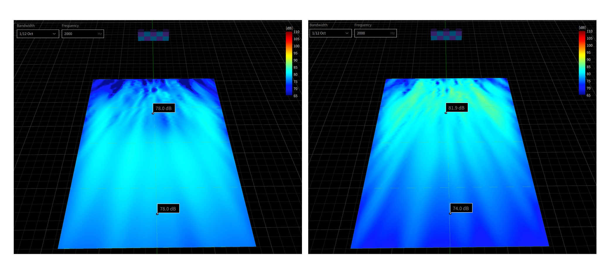 *Left - SPL Drop over Distance: 0 dB per distance doubling / Right - SPL Drop over Distance: 6 dB per distance doubling*
## Beam variant-specific parameters
Below the general parameters, you'll find the Coverage Beam parameters which are specific to the beam variant. Only one version of a beam variant can be used in a preset layer. Find out more in the Working with Beam Variants section.
{% content-ref url="/pages/URm8tkJDtyZoNWHOjoBe" %}
[Working with beam variants (advanced)](/holoplot-plan/working-with-beams/creating-a-coverage-beam/working-with-beam-variants-advanced)
{% endcontent-ref %}
Edit the following parameters and click **Optimize** to create a beam.
### Target response
Chooses a predefined frequency response for the optimization.\
\
By specifying the target frequency response curve for the optimization, you can effectively achieve the desired sound at the selected audience zone, saving time (and headroom) during the tuning phase. Defining the system frequency response using the target response will automatically adjust the DSP chain (up or down) to reach 0 dB headroom in any passbands. Alternatively, using a parametric EQ on the beam might overdrive the system, causing a lack of headroom, or underuse it, resulting in excess headroom. Consequently, using the target response makes the most out of the available headroom, allowing for a more efficient tuning process. You can select the target response from a list of predefined curves:
* Flat
* Low-shelf +7 dB
* Low-shelf +6 dB
* Low-shelf +3 dB
* High-shelf +9 dB
* High-shelf +6 dB
* High-shelf +3 dB
 
### Phase Response
The Phase Response feature in HOLOPLOT Plan allows you to choose the phase behavior of the Coverage Beam, effectively adjusting the group delay of the array's different passbands.
There are four different phase response options available:
*Left - SPL Drop over Distance: 0 dB per distance doubling / Right - SPL Drop over Distance: 6 dB per distance doubling*
## Beam variant-specific parameters
Below the general parameters, you'll find the Coverage Beam parameters which are specific to the beam variant. Only one version of a beam variant can be used in a preset layer. Find out more in the Working with Beam Variants section.
{% content-ref url="/pages/URm8tkJDtyZoNWHOjoBe" %}
[Working with beam variants (advanced)](/holoplot-plan/working-with-beams/creating-a-coverage-beam/working-with-beam-variants-advanced)
{% endcontent-ref %}
Edit the following parameters and click **Optimize** to create a beam.
### Target response
Chooses a predefined frequency response for the optimization.\
\
By specifying the target frequency response curve for the optimization, you can effectively achieve the desired sound at the selected audience zone, saving time (and headroom) during the tuning phase. Defining the system frequency response using the target response will automatically adjust the DSP chain (up or down) to reach 0 dB headroom in any passbands. Alternatively, using a parametric EQ on the beam might overdrive the system, causing a lack of headroom, or underuse it, resulting in excess headroom. Consequently, using the target response makes the most out of the available headroom, allowing for a more efficient tuning process. You can select the target response from a list of predefined curves:
* Flat
* Low-shelf +7 dB
* Low-shelf +6 dB
* Low-shelf +3 dB
* High-shelf +9 dB
* High-shelf +6 dB
* High-shelf +3 dB
 
### Phase Response
The Phase Response feature in HOLOPLOT Plan allows you to choose the phase behavior of the Coverage Beam, effectively adjusting the group delay of the array's different passbands.
There are four different phase response options available: